In this blog post, I explore concepts around separable convolutional image filters: how can we check if a 2D filter (like convolution, blur, sharpening, feature detector) is separable, and how to compute separable approximations to any arbitrary 2D filter represented in a numerical / matrix form. I’m not covering any genuinely new research, but think it’s a really cool, fun, visual, interesting, and very practical topic, while being mostly unknown in the computer graphics community.

Throughout this post, will explore some basic use of Singular Value Decomposition, one of the most common and powerful linear algebra concepts (used in all sub-fields of computer science, from said image processing, through recommendation systems, ML, to ranking web pages in search engines). We will see how it can be used to analyze 2D image processing filters – check if they are separable, approximate the non-separable ones, and will demonstrate how to use those for separable, juicy bokeh.

Note: this post turned out to be a part one of a mini-series, and has a follow-up post here – be sure to check it out!

Post update: Using separable filters for bokeh approxmation is not a new idea – Olli Niemitalo pointed out this paper “Fast Bokeh effects using low-rank linear filters” to me, which doesn’t necessarily feature any more details on the technique, but has some valuable timings/performance/quality comparisons to the stochastic sampling, if you are interested in using it in practice, check it out – along my follow-up post.

Intro / motivation

Separable filters are one of the most useful tools in image processing and they can turn algorithms from “theoretical and too expensive” to practical under the same computational constraints. In some other cases, ability to use a separable filter can be the tipping point that makes some “interactive” (or offline) technique real-time instead.

Let’s say we want to filter an image – sharpen it, blur, maybe detect the edges or other features. Given a 2D image filter of size MxN, computing the filter would require MxN independent, sequential memory accesses (often called them “taps”), accompanied by MxN multiply-add operations. For large filters, this can get easily prohibitively expensive, and we get quadratic scaling with the filter spatial extent… This is where separable filters can come to the rescue.

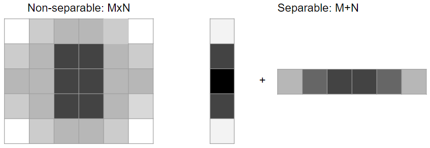
If a filter is separable, we can decompose such filter into a sequence of two 1D filters in different directions (usually horizontal, and then vertical). Each pass filters with a 1D filter, first with M, and then the second pass with N taps, in total M+N operations. This requires storing the intermediate results – either in memory, or locally (line buffering, tiled local memory optimizations). While you pay the cost of storing the intermediate results and synchronizing the passes, you get linear and not quadratic scaling. Therefore, typically for any filter sizes larger than ~4×4 (depends on the hardware, implementation etc) using separable filters is going to be significantly faster than the naive, non-separable approach.

But how do we find separable filters?

Simplest analytical filters

Two simplest filters that are bread and butter of any image processing are the box filter, and the Gaussian filter. Both of them are separable, but why?

The box filter seems relatively straightforward – there are two ways of thinking about it: a) if you intuitively think about what happens if you just “smear” a value across horizontal, and then vertical axis, you will get a box; b) mathematically, there are two conditions on the value of the filter, there are two conditions on both dimensions that are independent:

f(x, y) = select(abs(x) < extent_x && abs(y) < extent_y), v, 0)
f(x, y) = select(abs(x) < extent_x, v, 0) * select(abs(y) < extent_y, 1, 0) 

This last product is the equation of separability – our 2D function is a product of a horizontal, and a vertical function.

Gaussian is a more interesting one, and it’s not immediately obvious (“what does the normal distribution have to do with separability?”), so let’s write out the maths.

For simplicity, I will use a non-normalized Gaussian function (usually we need to re-normalize after the discretization anyway) and assume standard deviation of 1/sqrt(2) so that it “disappears” from the denominator.

f(x, y) = exp(-sqrt(x^2 + y^2)^2) // sqrt(x^2 + y^2) is distance of filtered pixel
f(x, y) = exp(-(x^2 + y^2))       // from the filter center.
f(x, y) = exp(-x^2 + -y^2)
f(x, y) = exp(-x^2) * exp(-y^2)

The last step follows from the “definition” of exponential (exponential of sum is a product of exponentials), and afterwards we can see that again, our 2D filter is product of two 1D Gaussian filters.

“Numerical” / arbitrary filters

We started with two trivial, analytical filters, but what do we do if we have an arbitrary filter given to us in a numerical form – just a matrix full of numbers?

We can plot them, analyze them, but how do we check if given filter is separable? Can we try to separate (maybe at least approximately) any filter?

Linear algebra to the rescue

Let’s rephrase our problem in terms of linear algebra. Given a matrix MxN, we would like to express it as a product of two matrices, Mx1 and 1xN. Let’s re-draw our initial diagram:

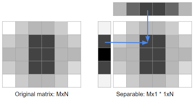
There are a few ways of looking at this problem (they are roughly equivalent – but writing them all out should help build some intuition for it):

• We would like to find a row Mx1 that can be replicated with different multipliers N times giving us original matrix,
• Another way of saying the above is that we would like our MxN filter matrix rows/columns to be linearly dependent,
• We would like our source matrix to be a matrix with rank of one,
• If it’s impossible, then we would like to get a low-rank approximation of the matrix MxN.

To solve this problem, we will use one of the most common and useful linear algebra tools, Singular Value Decomposition.

Proving that it gives “good” results (optimal in least-squarest sense, at least for some norms) is beyond the scope of this post, but if you’re curious, check out the proofs on the wikipedia page.

Singular Value Decomposition

Specifically, the singular value decomposition of an  real or complex matrix  is a factorization of the form , where  is an  real or complex unitary matrix, is an rectangular diagonal matrix with non-negative real numbers on the diagonal, and  is an  real or complex unitary matrix. If  is real,  and  are real orthonormal matrices.

Wikipedia

How does SVD help us here? We can look at the final matrix as a sum of many matrix multiplications, each of a single row/column from the U and V matrix, multiplied by the diagonal entry from the matrix E. SVD diagonal matrix E contains entries (called “singular values”) on the diagonal only and they are sorted from the highest value, to the lowest. If we look at the final matrix as a sum of different rank 1 matrices, weighted by their singular values, the singular values correspond to proportion of the “energy”/”information” of the original matrix contents.

If our original matrix is separable, then it is rank 1, and we will have only single singular value. Even if they are not zero (but significantly smaller), and we truncate all coefficients except for the first one, we will get a separable approximation of the original filter matrix!

Note: SVD is a concept and type of matrix factorization / decomposition, not an algorithm to compute one. Computing SVD efficiently and numerically stable is generally difficult (requires lots of careful consideration) and I am not going to cover it – but almost every linear algebra package or library has it implemented, and I assume we just use one.

Simple, separable examples

Let’s start with our two simple examples that we know that are separable – box and Gaussian filter. We will be using Python and numpy / matplotlib. This is just a warm-up, so feel free to skip those two trivial cases and jump to the next section.

import numpy as np
import matplotlib.pyplot as plt
import scipy.ndimage
plt.style.use('seaborn-whitegrid')

x, y = np.meshgrid(np.linspace(-1, 1, 50), np.linspace(-1, 1, 50))
box = np.array(np.logical_and(np.abs(x) < 0.7, np.abs(y) < 0.7),dtype='float64') 
gauss = np.exp(-5 * (x * x + y * y))
plt.matshow(np.hstack((gauss, box)), cmap='plasma')
plt.colorbar()

Let’s see what SVD will do with the box filter matrix and print out all the singular values, and and the U and E row / column associated with the first singular value:

U, E, V = np.linalg.svd(box)
print(E)
print(U[:,0])
print(V[0,:])

[34.00 0.00 0.00 0.00 0.00 0.00 0.00 0.00 0.00 0.00 0.00 0.00 0.00 0.00
 0.00 0.00 0.00 0.00 0.00 0.00 0.00 0.00 0.00 0.00 0.00 0.00 0.00 0.00
 0.00 0.00 0.00 0.00 0.00 0.00 0.00 0.00 0.00 0.00 0.00 0.00 0.00 0.00
 0.00 0.00 0.00 0.00 0.00 0.00 0.00 0.00]
[0.00 0.00 0.00 0.00 0.00 0.00 0.00 0.00 -0.17 -0.17 -0.17 -0.17 -0.17
 -0.17 -0.17 -0.17 -0.17 -0.17 -0.17 -0.17 -0.17 -0.17 -0.17 -0.17 -0.17
 -0.17 -0.17 -0.17 -0.17 -0.17 -0.17 -0.17 -0.17 -0.17 -0.17 -0.17 -0.17
 -0.17 -0.17 -0.17 -0.17 -0.17 0.00 0.00 0.00 0.00 0.00 0.00 0.00 0.00]
[0.00 0.00 0.00 0.00 0.00 0.00 0.00 0.00 -0.17 -0.17 -0.17 -0.17 -0.17
 -0.17 -0.17 -0.17 -0.17 -0.17 -0.17 -0.17 -0.17 -0.17 -0.17 -0.17 -0.17
 -0.17 -0.17 -0.17 -0.17 -0.17 -0.17 -0.17 -0.17 -0.17 -0.17 -0.17 -0.17
 -0.17 -0.17 -0.17 -0.17 -0.17 0.00 0.00 0.00 0.00 0.00 0.00 0.00 0.00]

Great, we get only one singular value – which means that it is a rank 1 matrix and fully separable.

On the other hand, the fact that our columns / vectors are negative is a bit peculiar (it is implementation dependent), but the signs negate each other; so we can simply multiply both of them by -1. We can also get rid of the singular value and embed it into our filters, for example bymultiplying both by sqrt of it to make them comparable in value:

[-0.00 -0.00 -0.00 -0.00 -0.00 -0.00 -0.00 -0.00 1.00 1.00 1.00 1.00 1.00
 1.00 1.00 1.00 1.00 1.00 1.00 1.00 1.00 1.00 1.00 1.00 1.00 1.00 1.00
 1.00 1.00 1.00 1.00 1.00 1.00 1.00 1.00 1.00 1.00 1.00 1.00 1.00 1.00
 1.00 -0.00 -0.00 -0.00 -0.00 -0.00 -0.00 -0.00 -0.00]
[-0.00 -0.00 -0.00 -0.00 -0.00 -0.00 -0.00 -0.00 1.00 1.00 1.00 1.00 1.00
 1.00 1.00 1.00 1.00 1.00 1.00 1.00 1.00 1.00 1.00 1.00 1.00 1.00 1.00
 1.00 1.00 1.00 1.00 1.00 1.00 1.00 1.00 1.00 1.00 1.00 1.00 1.00 1.00
 1.00 -0.00 -0.00 -0.00 -0.00 -0.00 -0.00 -0.00 -0.00]

Apart from cute -0.00s, we get exactly the separable filter we would expect. We can do the same with the Gaussian filter matrix and arrive at the following:

[0.01 0.01 0.01 0.02 0.03 0.04 0.06 0.08 0.10 0.14 0.17 0.22 0.27 0.33
 0.40 0.47 0.55 0.63 0.70 0.78 0.84 0.90 0.95 0.98 1.00 1.00 0.98 0.95
 0.90 0.84 0.78 0.70 0.63 0.55 0.47 0.40 0.33 0.27 0.22 0.17 0.14 0.10
 0.08 0.06 0.04 0.03 0.02 0.01 0.01 0.01]
[0.01 0.01 0.01 0.02 0.03 0.04 0.06 0.08 0.10 0.14 0.17 0.22 0.27 0.33
 0.40 0.47 0.55 0.63 0.70 0.78 0.84 0.90 0.95 0.98 1.00 1.00 0.98 0.95
 0.90 0.84 0.78 0.70 0.63 0.55 0.47 0.40 0.33 0.27 0.22 0.17 0.14 0.10
 0.08 0.06 0.04 0.03 0.02 0.01 0.01 0.01]

Now if we take an outer product (using function np.outer()) of those two vectors, we arrive at filters almost exactly same as the original (+/- the numerical imprecision differences).

Non-separable filters

“D’oh, you took filters that you know are separable, fed through some complicated linear algebra machinery and verified that yes, they are separable – what a waste of time!” you might think – and you are right, it was a demonstration of the concept, but has so far not too much practical value. So let’s look at a few more interesting filters – ones that we know are not separable, but maybe are almost separable?

I picked four examples: circular, hexagon, exponential/Laplace distribution, and a difference of Gaussians. Circular and hexagon are interesting as they are very useful for bokeh; exponential/Laplace is somewhat similar to long-tailed BRDF like GGX, and can be used for some “glare”/veil type of effects, and the difference of Gaussians (laplacian of Gaussians) is both a commonly used band-pass filter, as well as can be used for a busy, “donut”-type bokeh.

circle = np.array(x*x+y*y < 0.8, dtype='float64')
exponential = np.exp(-3 * np.sqrt(x*x+y*y))

hexagon = np.array(np.logical_and(np.logical_and(np.logical_and(np.logical_and(np.logical_and(np.logical_and(np.logical_and(x+y < 0.9*np.sqrt(2), x+y > -0.9*np.sqrt(2)),x-y < 0.9*np.sqrt(2)),-x+y < 0.9*np.sqrt(2)),x<0.9),x>-0.9),y<0.9),y>-0.9), dtype='float64')

difference_of_gaussians = np.exp(-5 * (x*x+y*y))-np.exp(-6 * (x*x+y*y))
difference_of_gaussians /= np.max(difference_of_gaussians)

plt.matshow(np.vstack((np.hstack((circle, hexagon)), np.hstack((exponential, difference_of_gaussians)))), cmap='plasma')
plt.colorbar()

Now, if we try to do a rank 1 approximation by taking just the first singular value, we end up with results looking like this:

They look terrible, nothing like the original ones! Ok, so now we know they are not separable, which concludes my blog post…

I’m obviously kidding, let’s explore how “good” are those approximations and how to make them better. 🙂

Low~ish rank approximations

I mentioned that singular values represent percentage of “energy” or “information” in the original filter. If the filter is separable, all energy is in the first singular value. If it’s not, then it will be distributed among multiple singular values.

We can plot the magnitude of singular values (I normalized all the plots so they integrate to 1 like a density function and don’t depend on how bright a filter is) to see what is going on. Here are two plots: of the singular values, and “cumulative” (reaching 1 means 100% of the original filter preserved). There are 50 singular values in a 50×50 matrix, but after some point they reach zero, so I truncated the plots.

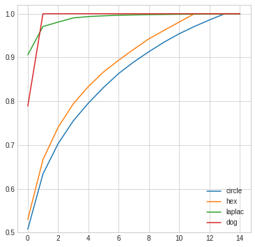
The second plot is very informative and tells us what we can expect from those low rank approximations.

To reconstruct fully the original filter, for difference of Gaussians we need just two rank 1 matrices (this is not surprising at all! DoG is difference of two Gaussians, separable / rank 1 filters), for Laplacian we get very close with just 2-3 rank 1 matrices. On the other hand, for circular and hexagonal filter we need many more, to reach just 75% accuracy we need 3-4 filters, and 14 to get 100% accurate representation…

How do such higher rank approximations look like? You can think of them as sum of N independent separable filters (independent vertical + horizontal passes). In practice, you would probably implement them as a single horizontal pass that produces N outputs, followed by a vertical one that consumes those, multiplies them with appropriate vertical filters, and produces a single output image.

Note 1: In general and in most cases, the “sharper” (like the immediate 0-1 transition of hex or a circle) or less symmetric a filter is, the more difficult it will be to approximate it. In a way, it is similar to other common decomposition, like the Fourier transform.

Note 2: You might wonder – if a DoG can be expressed as a sum of two trivially separable Gaussians, why SVD rank 1 approximation doesn’t look like one of the Gaussians? The answer is that with just a single Gaussian, the resulting filter will be more different from the source than our separable weird 4-dot pattern. SVD decomposes so that each progressive low rank decomposition is optimal (in L2 sense), in this case it means adding two non-intuitive, “weird” separable patterns together, where the second one contributes 4x less than the first one.

Low-rank approximations in practice

Rank N approximation of an MxM filter would have performance cost of O(2M*N), but additional memory cost of N * original image storage (if not doing any common optimizations like line buffering or local/tiled storage). If we need to approximate 50×50 filter, then even taking 10 components could be “theoretically” worth it; and for much larger filters it would be also worth in practice (and still faster and less problematic than FFT based approaches). One thing worth noting is that in the case of presented filters, we reach the 100% exact accuracy with just 14 components (as opposed to full 50 singular values!).

But let’s look at more practical, 1, 2, 3, 4 component approximations.

def low_rank_approx(m, rank = 1):
  U,E,V = np.linalg.svd(m)
  mn = np.zeros_like(m)
  score = 0.0
  for i in range(rank):
    mn += E[i] * np.outer(U[:,i], V[i,:])
    score += E[i]
  print('Approximation percentage, ', score / np.sum(E))
  return mn

Even with those maximum four components, we see a clear “diminishing returns” effect, and that the differences get smaller between 3 and 4 components as compared to 2 and 3. This is not surprising, since our singular values are sorted descending, so every next approximation will add less of information. Looking at the results, they might be actually not too bad. We see some “blockiness”, and even worse negative values (“ringing”), but how would that perform on real images?

Visual effect of low-rank approximation – boookeh!

To demonstrate how good/bad this works in practice, I will use filters to blur an image (from the Kodak dataset). On LDR images the effects are not very visible, so I will convert it to fake HDR by applying a strong gamma function of 7, doing the filtering, and inverse gamma 1/7 to emulate tonemapping. It’s not the same as HDR, but does the job. 🙂 This will also greatly amplify any of the filter problems/artifacts, which is what we want for the analysis – with approximations we often want to understand not just the average, but also the worst case.

def fake_tonemap(x):
  return np.power(np.clip(x, 0, 1), 1.0/7.0)
def fake_inv_tonemap(x):
  return np.power(np.clip(x, 0, 1), 7.0)
def filter(img, x):
  res = np.zeros_like(img)
  for c in range(3):
    # Note that we normalize the filter to preserve the image brightness.
    res[:,:,c] = fake_tonemap(scipy.ndimage.convolve(fake_inv_tonemap(img[:,:,c]), x/np.sum(x)))
  return res
def low_rank_filter(img, x, rank = 1):
  final_res = np.zeros_like(img)
  U, E, V = np.linalg.svd(x / np.sum(x))
  for c in range(3):
    tmd = fake_inv_tonemap(img[:,:,c])
    for i in range(rank):
      final_res[:,:,c] += E[i] * scipy.ndimage.convolve(scipy.ndimage.convolve(tmd, U[:, i, np.newaxis]), np.transpose(V[i,:, np.newaxis]))
    final_res[:,:,c] = fake_tonemap(final_res[:,:,c])
  return final_res

Without further ado, here are the results.

Unsurprisingly, for the difference of Gaussians and exponential distribution, two components are enough to get identical filtered result, or very close to.

For the hexagon and circle, even 4 components show some of the negative “ringing” artifacts (bottom of the image), and one needs 8 to get artifact-free approximation. At the same time, we are using extreme gamma to show those shapes and emphasize the artifacts. Would this matter in practice and would such approximations be useful? As usually, it depends on the context of the filter, image content, further processing etc. I will put together some thoughts / recommendations in the Conclusions section.

A careful reader might ask – why not clamp filters to not be negative? The reason is that low rank approximations will often locally “overshoot” and add more energy in certain regions, so the next rank approximation component needs to remove it. And since we do it separably and accumulate the filtered result (the whole point of low rank approximation!) we don’t know if the sum will be locally negative or not. We could try to find some different, guaranteed non-negative decomposition, but it’s a NP-hard problem and only some approximations / heuristics / optimization-based solutions exist. Note: I actually wrote a blog post on using optimization to solve (or at least minimize) those issues as a follow-up, be sure to check it out! 🙂

Limitation – only horizontal/vertical separability

Before I conclude my post, I wanted to touch two related topics – one being a disadvantage of the SVD-based decomposition, the other one being a beneficial side-effect. Starting with the disadvantage – low-rank approximation in this context is limited to filters represented as matrices and strictly horizontal-vertical separability. This is very limited, as some real, practical, and important applications are not covered by it.

Let’s analyze two use-cases – oriented, orthogonal separability, and non-orthogonal separability. Anisotropic Gaussians are trivially separable with two orthogonal filter – along the principal direction, and perpendicular to it. Similarly, skewed box blur filters are separable, but in this case we need to blur in two non-orthogonal directions. (Note: this separability is the basis of classic technique of fast hexagonal blur developed by John White and Colin Barre-Brisebois).

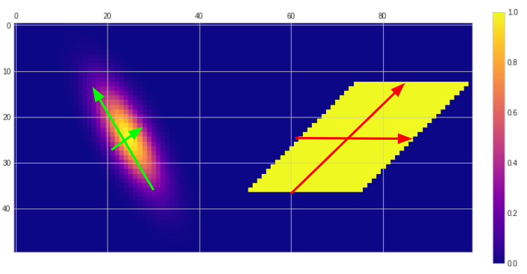
Such filtering can be done super-fast on the GPU, often almost as fast as the horizontal-vertical separation (depending if using texture sampler or compute shaders / local memory), yet the SVD factorization will not be able to find it… So let’s look at how the low rank horizontal-vertical approximations and accumulation of singular values look like.

Overall those approximations are pretty bad if you consider that they are trivially separable in those different direction. You could significantly improve them by finding the filter covariance principal components and rotate it to be axis aligned, but this is an approximation, requires filter resampling and complicates the whole process… Something to always keep in mind – as automatic linear algebra machinery (or any ML) is not a replacement for careful engineering and using the domain knowledge. 🙂

Bonus – filter denoising

My post is already a bit too long, so I will only hint at an interesting effect / advantage of SFV – how SVD is mostly robust to noise, and can be used for the filter denoising. If we take a pretty noisy Gaussian (Gaussian maximum of 1.0, noise standard deviation of 0.1), and do a simple rank1 decomposition, we get a significantly cleaner representation of it (albeit with horizontal and vertical “streaks”).

This approximation denoising efficacy will depend on the filter type; for example if we take our original circular filter (which is as we saw pretty difficult to approximate), the results are not going to be so great, as more components that would normally add more details, will add more noise back as well.

Therefore, there exists a point at which higher rank approximations will only add noise – as compared to adding back information/details. This is closely related to the bias-variance trade-off concept in machine learning, and we can see this behavior on the following plot showing normalized sum of squared error of the noisy circular filter next rank approximations (error is computed against ground truth, of non-noisy filter).

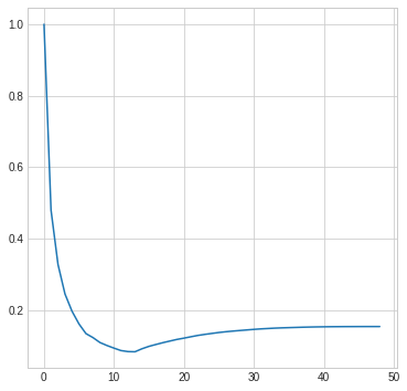
It is interesting to see on this plot that the cutoff point in this case is around rank 12-13 – while 14 components were enough to perfectly reconstruct the non-noisy version of the filter.

Overall this property of SVD is used in some denoising algorithms (however decomposed matrices are not 2D patches of an image; instead they usually are MxN matrices where M is a flattened image patch, representing all pixels in it as a vector, and N corresponds to N different, often neighboring or similar image patches), which is a super interesting technique, but way outside of the topic of this post.

Conclusions

To conclude, in this blog post we have looked at image filter/kernel separability – its computational benefits, simple and analytical examples, and shown a way of analyzing if a filter can be converted into a separable (rank 1) representation through Singular Value Decomposition.

As we encountered some examples of non-separable filters, we analyzed what are the higher rank approximations, how we can compute them through sum of many separable filters, how do they look like, and if we can apply them for image filtering using an example of bokeh.

I love the scientific and analytical approach, but I’m also an engineer at heart, so I cannot leave such blog post without answering – is it practical? When would someone want to use it?

My take on that is – this is just another tool in your toolbox, but has some immediate, practical uses. Those include analyzing and understanding your data, checking if some non-trivial filters can be separable, if they can be approximated despite the noise / numerical imprecision, and finally – evaluate how good the approximation is.

For non-separable filters, low rank approximations where the rank is higher than one can often be pretty good with just a few components and I think they are practical and usable. For example, our rank 4 approximation of the bokeh filters was not perfect (artifacts), but computationally way cheaper than non-separable filter, it parallelizes perfectly/trivially, and is very simple implementation-wise. In the past I referenced a very smart solution from Olli Niemitalo to approximate circular bokeh using complex phasors – and low-rank approximation in the real domain covered in this blog post is some simpler interesting alternative. Similarly, it might not produce perfect hexagonal blur like the one constructed using multiple skewed box filters, but the cost would be similar, and the implementation is so much simpler that it’s worth giving it a try.

I hope that this post was inspiring for some future explorations, understanding of the problem of separability, and you will be able to find some interesting, practical use-cases!