This paper is available on arxiv under CC 4.0 license.
Authors:
(1) Vianney Brouard, ENS de Lyon, UMPA, CNRS UMR 5669, 46 All´ee d’Italie, 69364 Lyon Cedex 07, France; E-mail: vianney.brouard@ens-lyon.f.
Table of Links
- Abstract & Introduction and presentation of the model
- Main results and biological interpretation
- First-order asymptotics of the mutant sub-populations for an infinite mono-directional grap
- First-order asymptotics of the mutant sub-populations for a general finite trait space (Theorem 2.1)
- Convergence for the stochastic exponents (Theorem 2.2)
- Acknowledgements & References
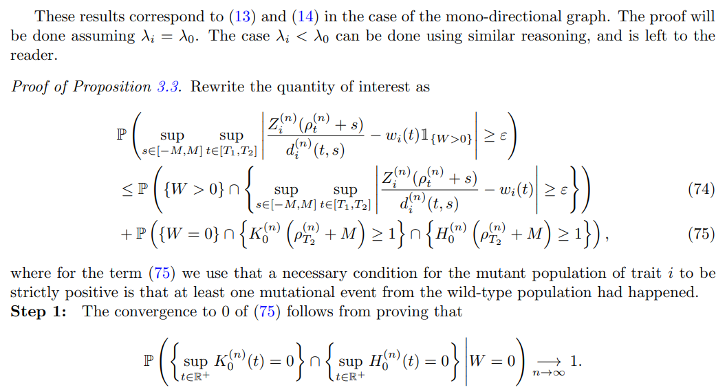
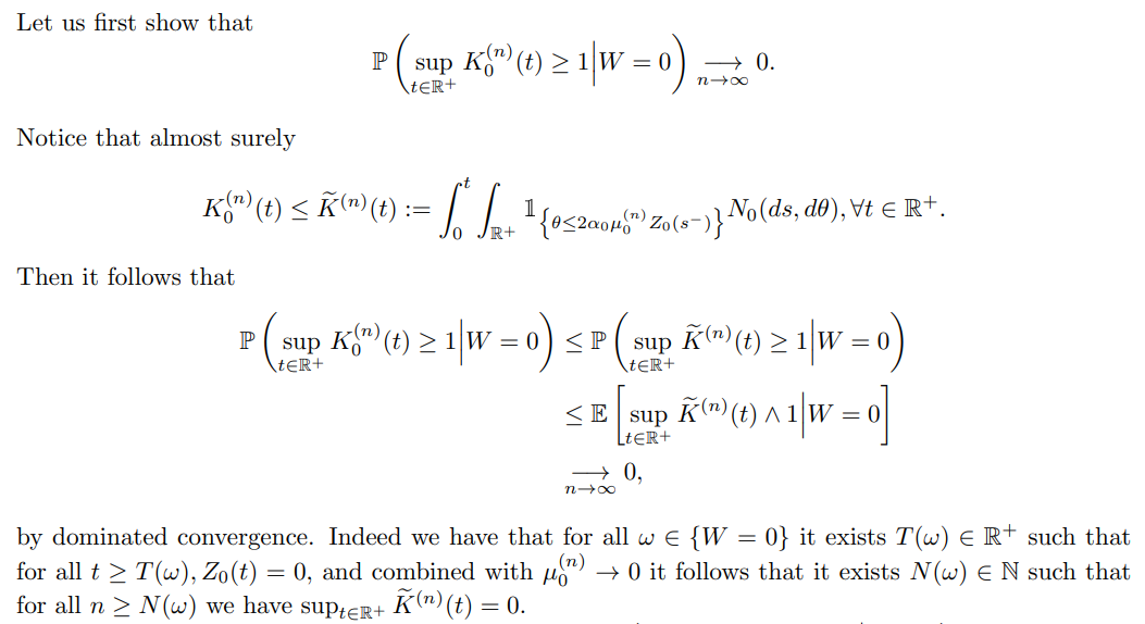
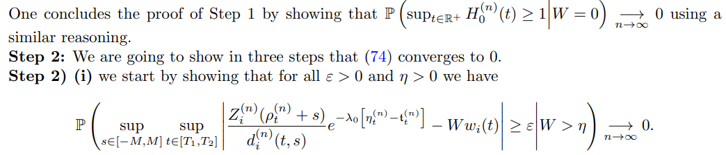
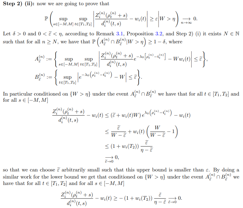
3 First-order asymptotics of the mutant sub-populations for an infinite mono-directional grap
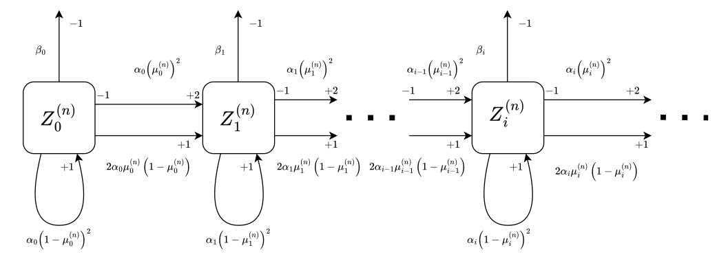
In this section consider the model described in Section 1 in the particular following infinite monodirectional grap
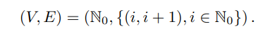
Assume in the case of the infinite mono-directional graph that

A graphical representation of the model can be found in Figure 5. In particular it means that any
Compared to the general finite graph, for any trait i ∈ N there is only one path from trait 0 to i for this mono-directional graph. In particular it implies that


Notice in particular that with such a construction it immediately follows the monotone coupling

Denote by
see [12] Section 1.1, or [11] Theorem 1.
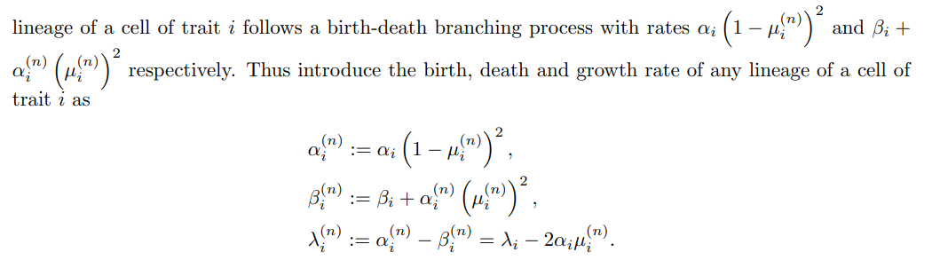
3.1 The wild-type dynamics

Using Ito’s formula and (18) it follows

Solving this equation we obtain for all t ≥ 0
Similarly we have
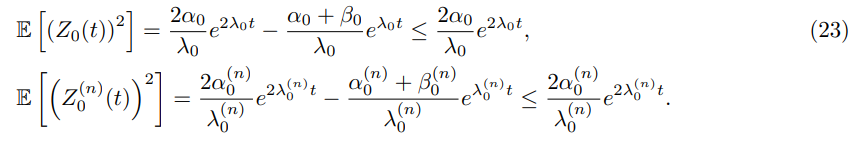
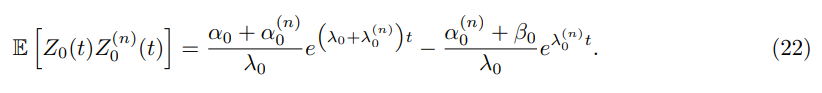
Consequently combining (21), (22) and (23) gives that
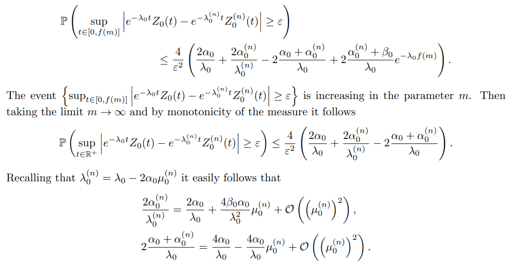
Finally we have

which concludes the proof.
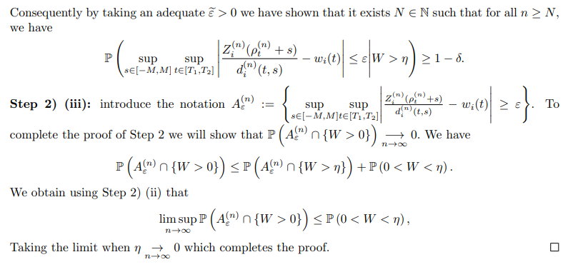
Proof of Lemma 3.2. Let ε > 0 and for all n ∈ N introduce the event
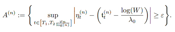
Step 1: We start by showing that for all 0 < δ1 < δ2
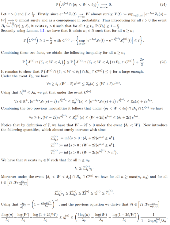
from which we obtain
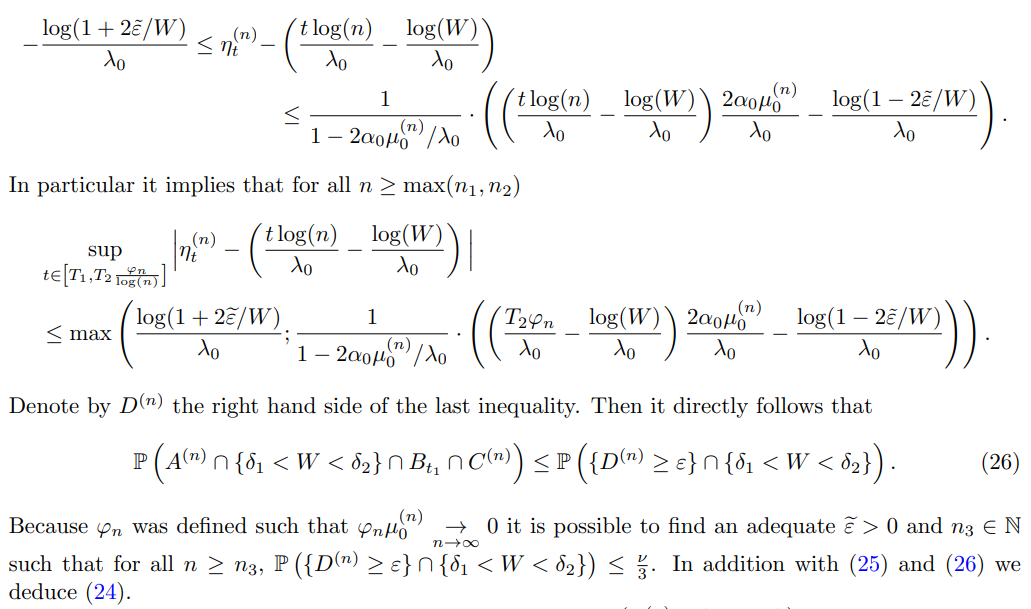
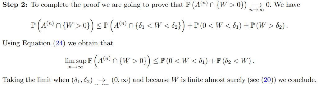
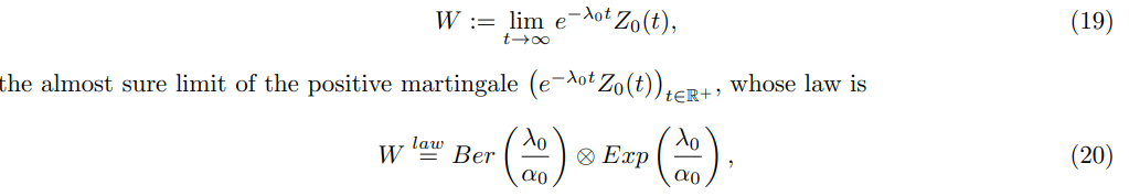
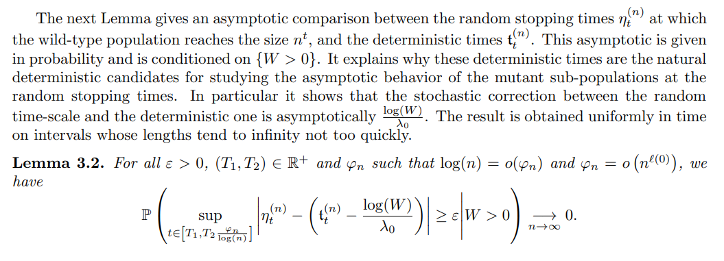
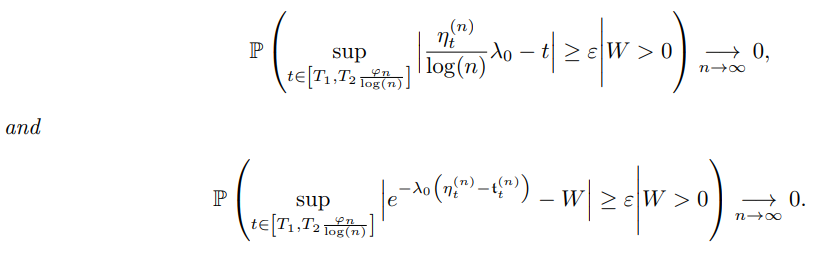
Remark 3.1. From Lemma 3.2, it follows the useful result
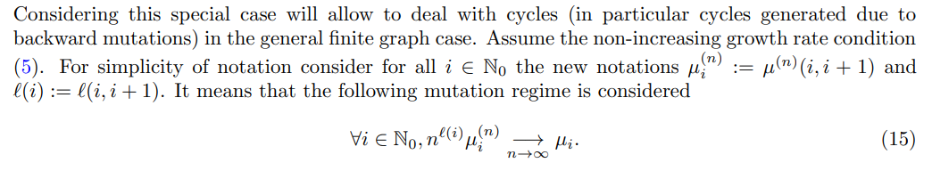
3.2 The mutant sub-populations dynamics in the deterministic time-scale (Theorem 2.1 (i))
In this subsection, Equations (11) and (12) are proven for the mono-directional graph. It will be done in two steps. The first one will consist in showing the result for a fixed s ∈ R and uniformly in the parameter t. Then in the second step, the result will be proved uniformly in the parameter
3.2.1 Uniform control on the time parameter
In this subsection we are going to prove the following proposition, which is a less refine result of (11) and (12), because the result is not uniform on the parameter s.
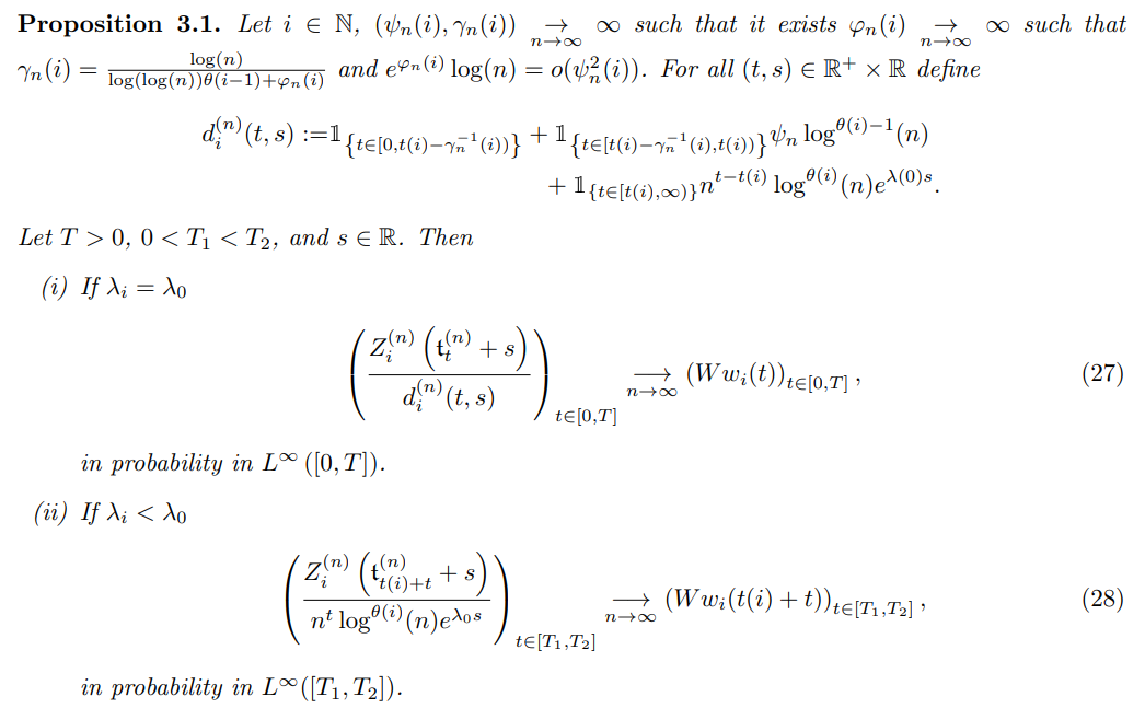
The proof is done by induction on i ∈ N. As long as the proof is similar for the initialization and the inductive part the step considered will not be specified. To make the proof the clearer possible it is cut using several lemmas.
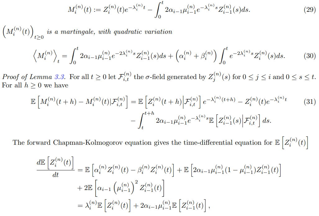
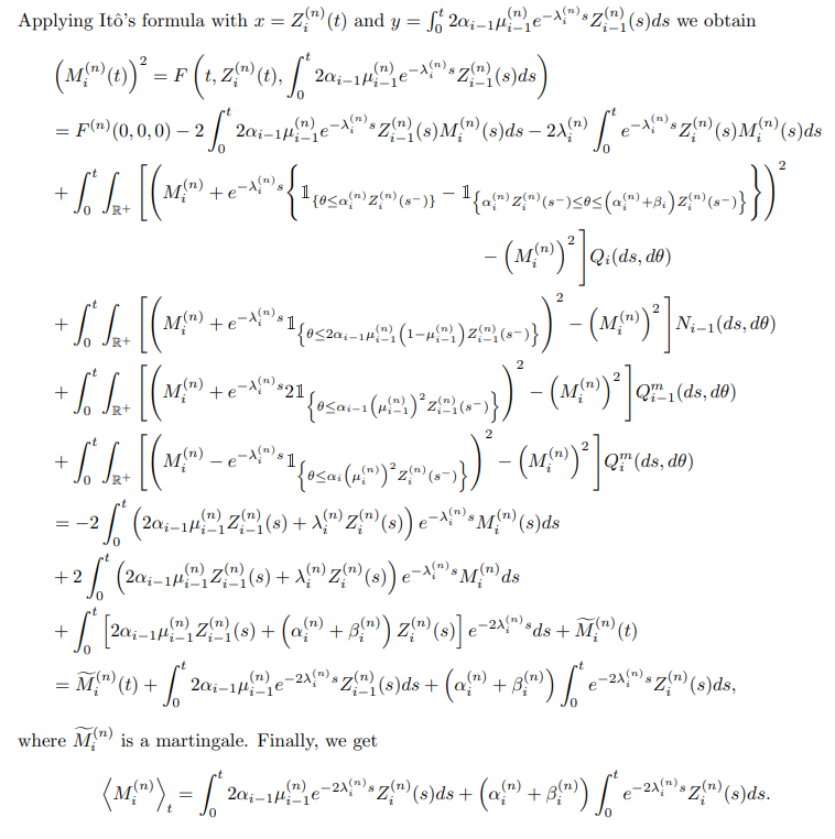
All the results are obtained using a martingale approach. In the next Lemma the martingales that are considered for all the mutant sub-populations are introduced, and their quadratic variations are computed.
Lemma 3.3. For all i ∈ N define

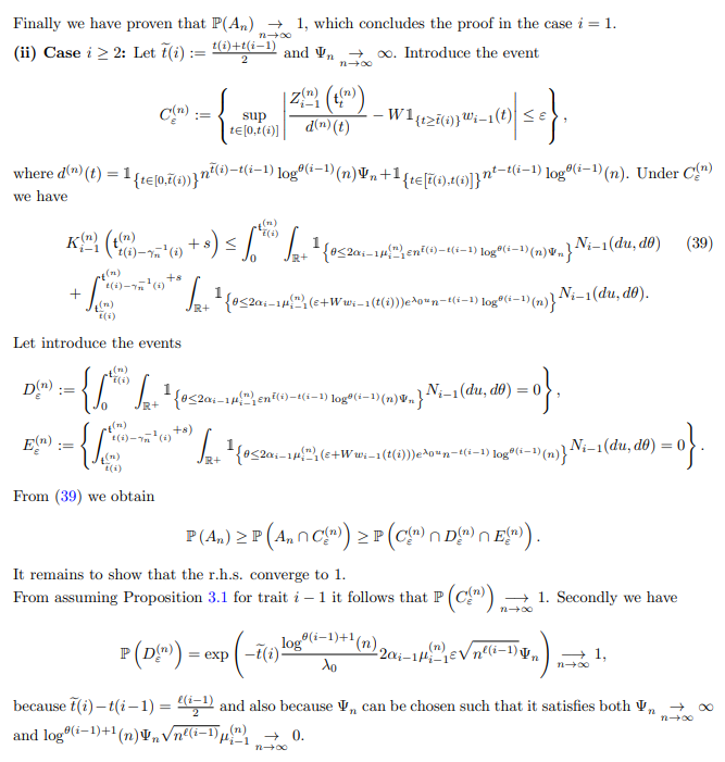
Proof of Proposition 3.1. Let i ∈ N ∗ . For i ≥ 2 assume that Proposition 3.1 is true for i − 1.
We start by showing the result when i is a neutral trait, that is to say we are going to prove (27). All the lemmas that we are mentioning in the proof are free from such neutral assumption, and work also for deleterious mutant traits.
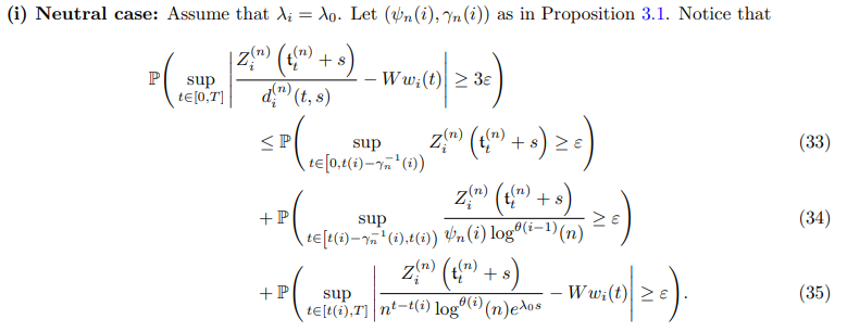
We are going to show that (33), (34) and (35) converges to 0 when n goes to infinity.
Step 1: Convergence to 0 of (33):

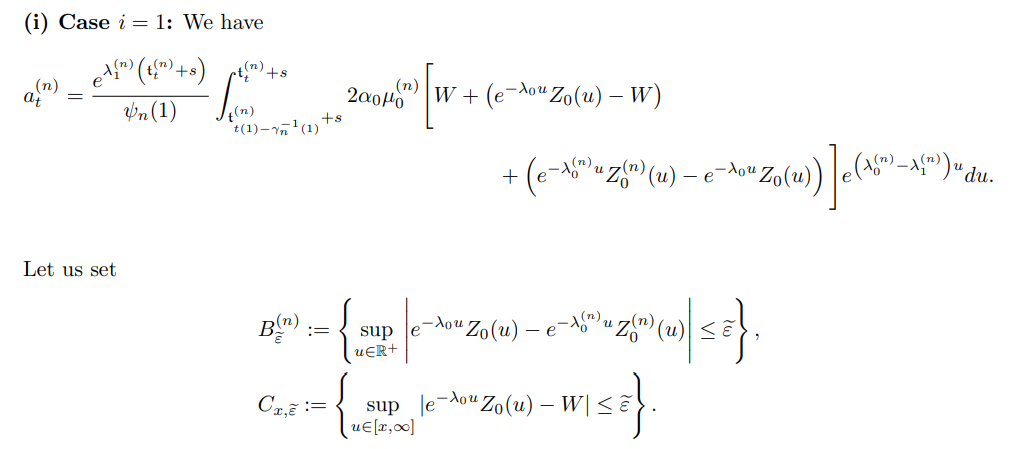
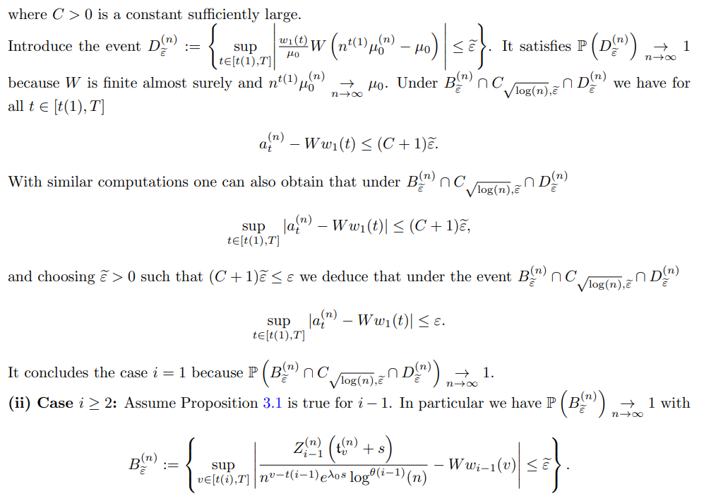
(i) Case i = 1:
Using Equation (38) we have that
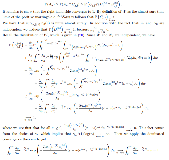


For i = 1 we prove (40) without condition.
It allows to write


For i = 1 we prove (44) without condition.
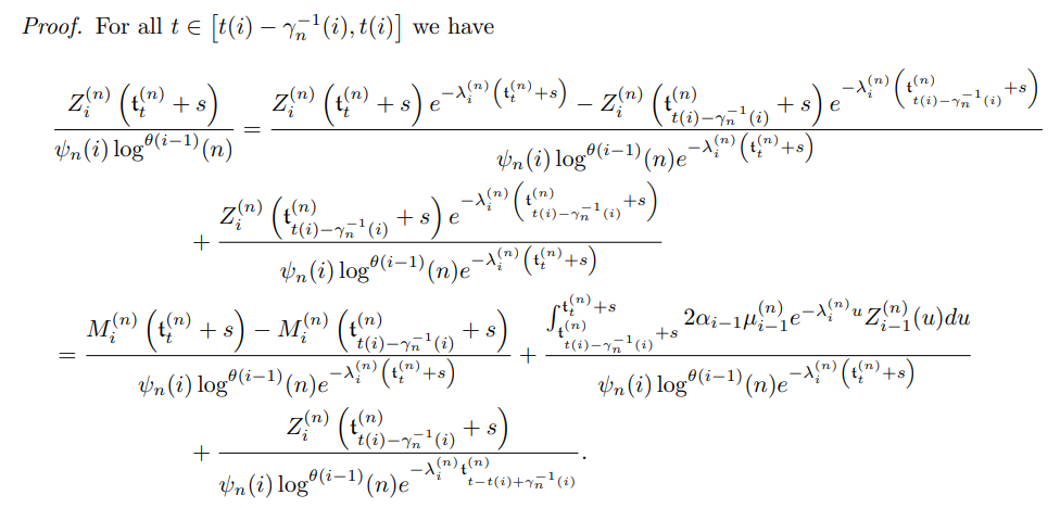
Proof of Lemma 3.6. Let
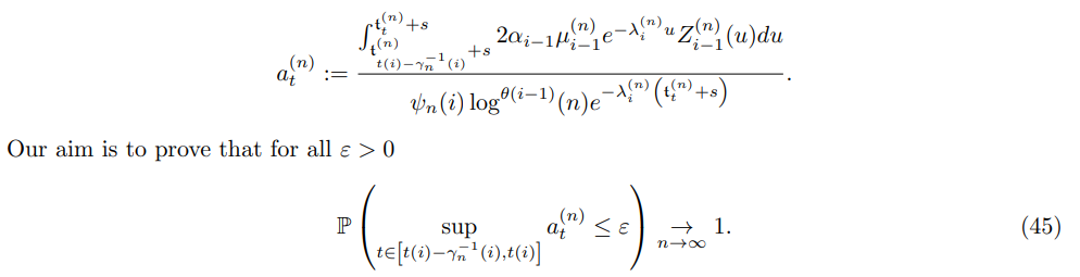


Using similar computations as in (46) and (47), it follows (45).

First, a natural upper bound on the mean of the growth of each mutant sub-population can be easily obtained. This is stated in the next Lemma.
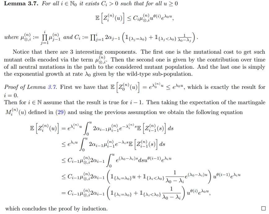
Second, using both the expression of the quadratic variation of the martingale associated to a mutant sub-population given in Equation (30) and the previous Lemma 3.7, a natural upperbound on its mean is obtained and summed up in the next Lemma.

First notice that the function
is a non-decreasing function implying that
Notice that
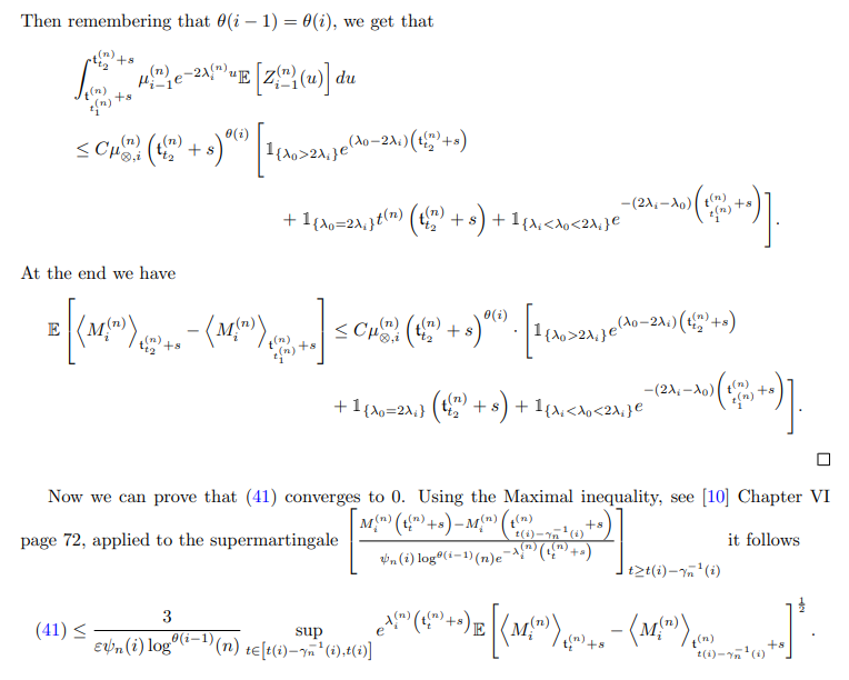
Then for n large enough, and remembering that θ(i) = θ(i − 1) + 1 we have

And we have
Then for n large enough, and remembering that θ(i) = θ(i − 1) we have

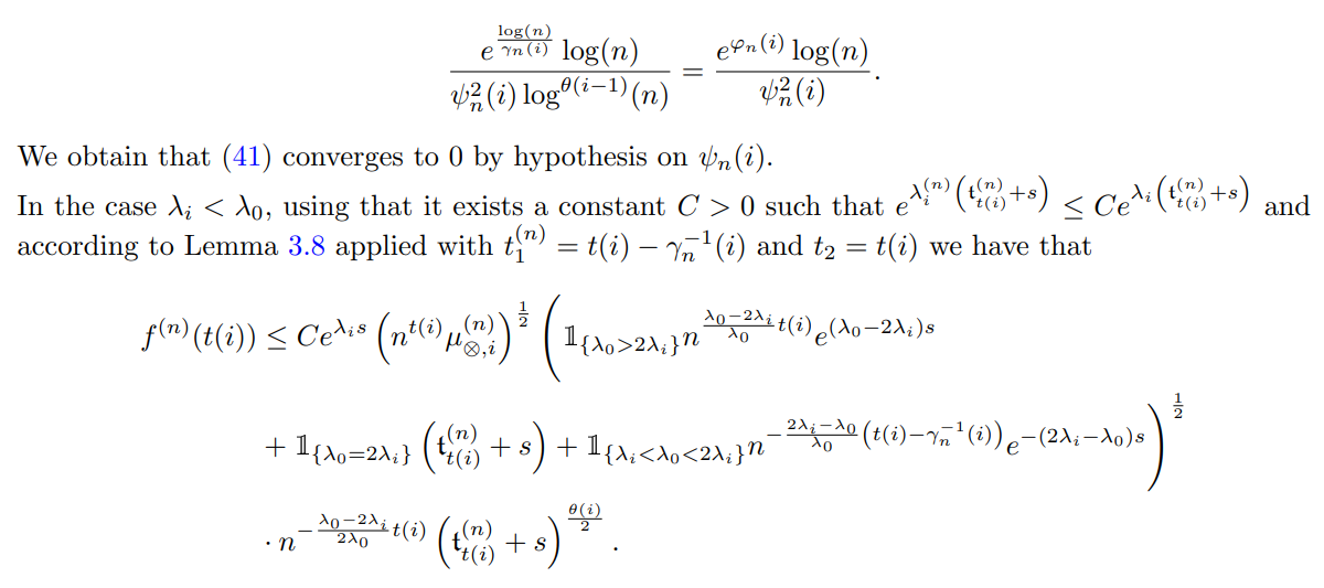
Then by hypothesis on (ψn(i), γn(i)) it follows that (41) converges to 0.
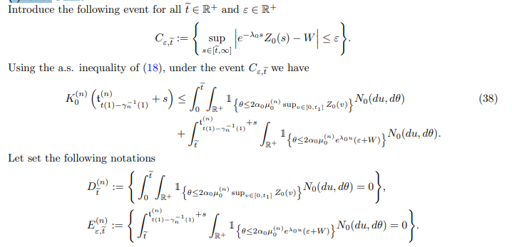
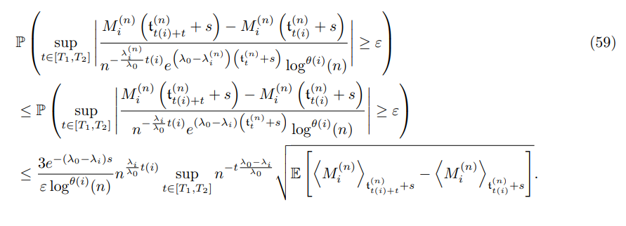
Step 3: Convergence to 0 of (35):
Notice that for all t ≥ t(i)

Then it allows to write


Then combining (52) and (53) we get

as θ(i) ≥ 1 since the vertex i is assumed to be neutral. It ends the proof of the convergence to 0 of the term (49).
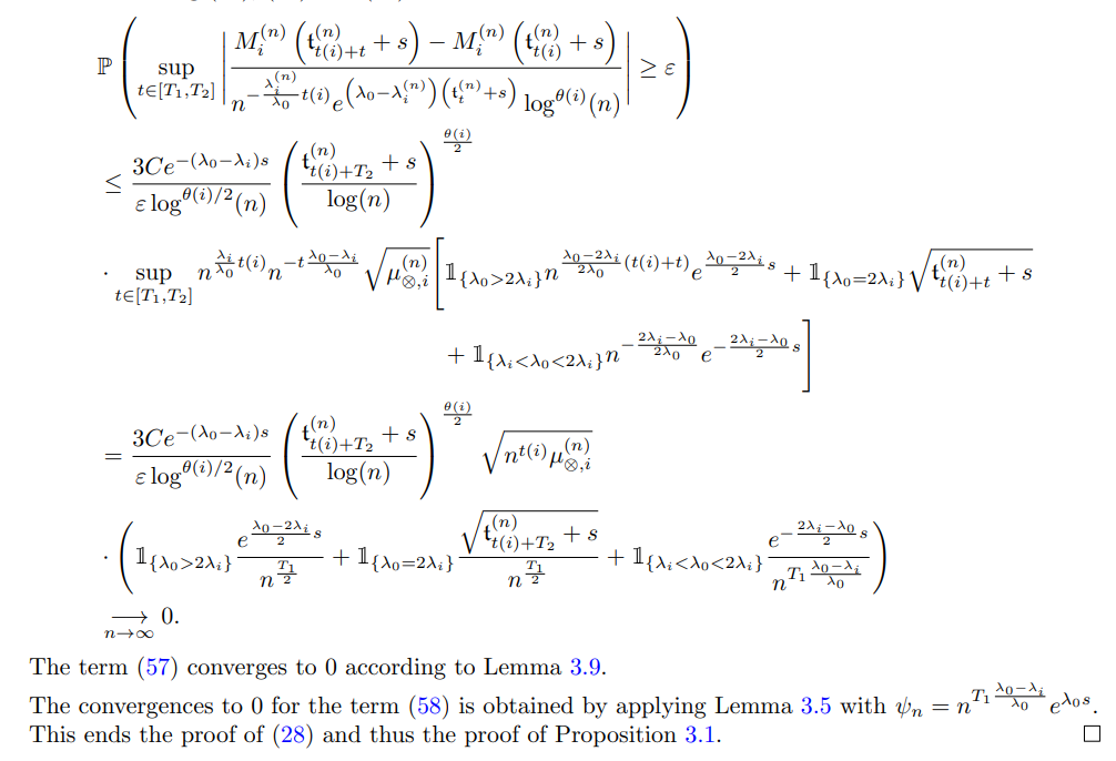
The term (50) converges to 0 according to the following Lemma.
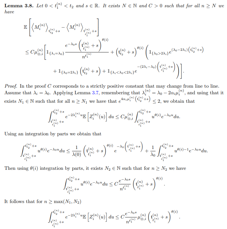
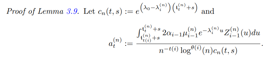
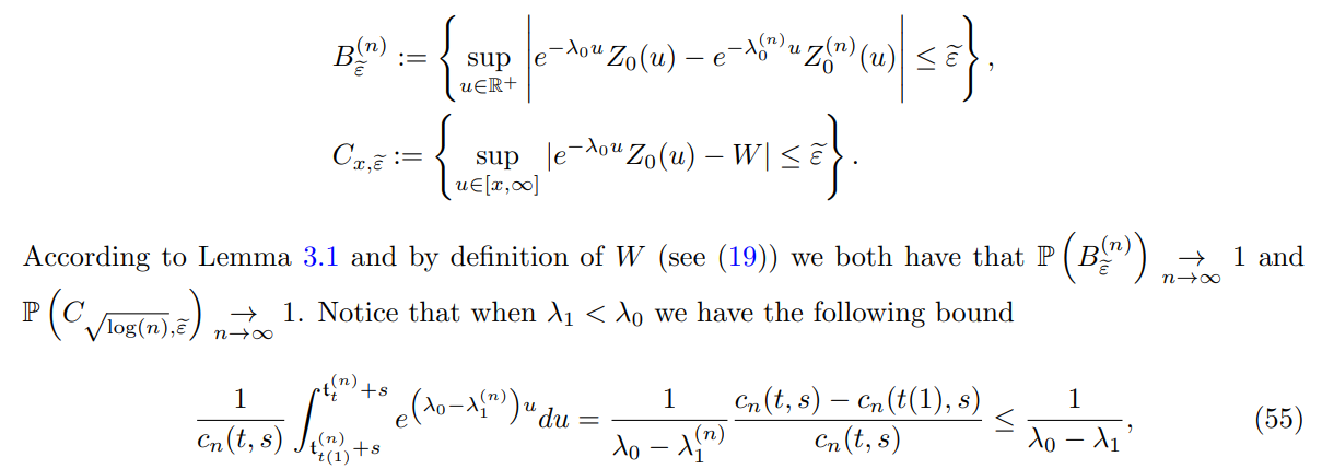
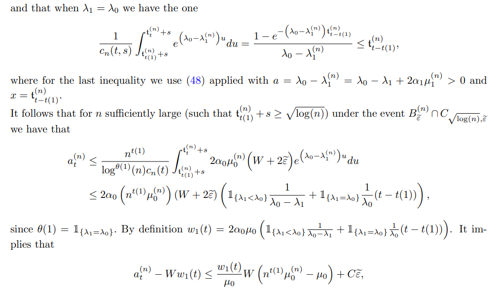
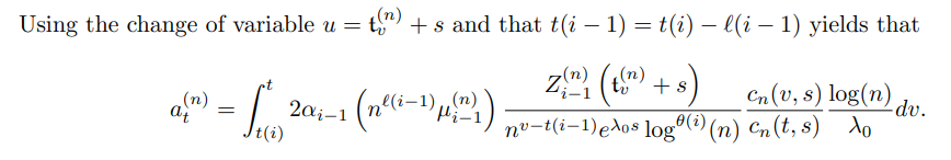
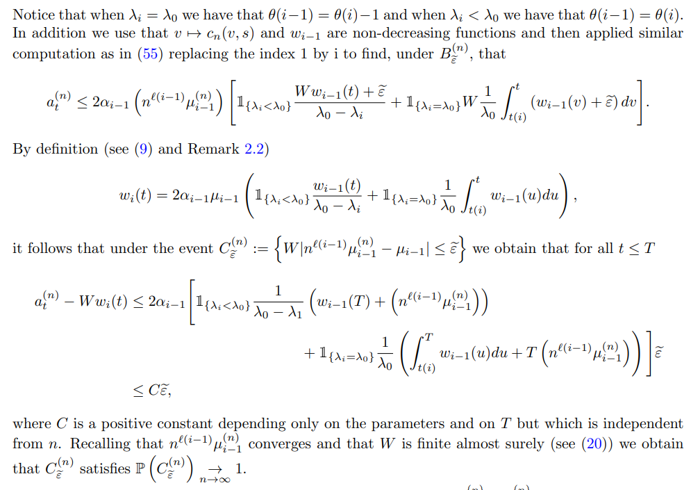
Lemma 3.9. Assume Equation (15). Let i ∈ N, T ≥ t(i) and s ∈ R. For i ≥ 2 we prove that if Proposition 3.1 is true for i − 1 then

For i = 1, we prove (54) without condition.
Our aim is to prove that for all ε > 0

(i) Case i = 1: We have
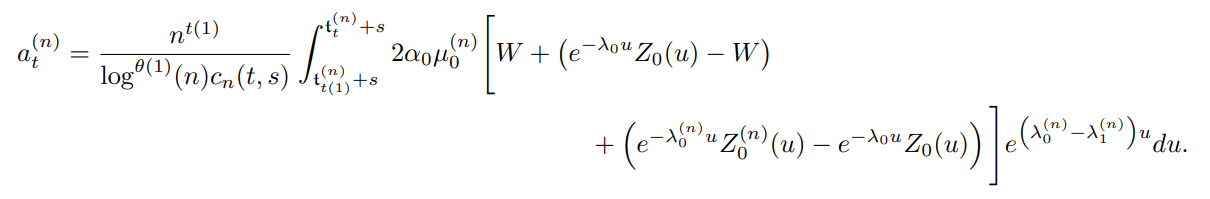
Let us set


3.2.2 Uniform control on the parameter s
In this subsection we will prove (11) and (12) from (27) and (28) using an idea from the proof of Lemma 3 of [15].
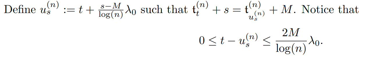
We start by showing (12). We will use that
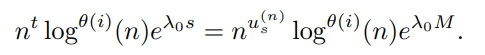
It gives that
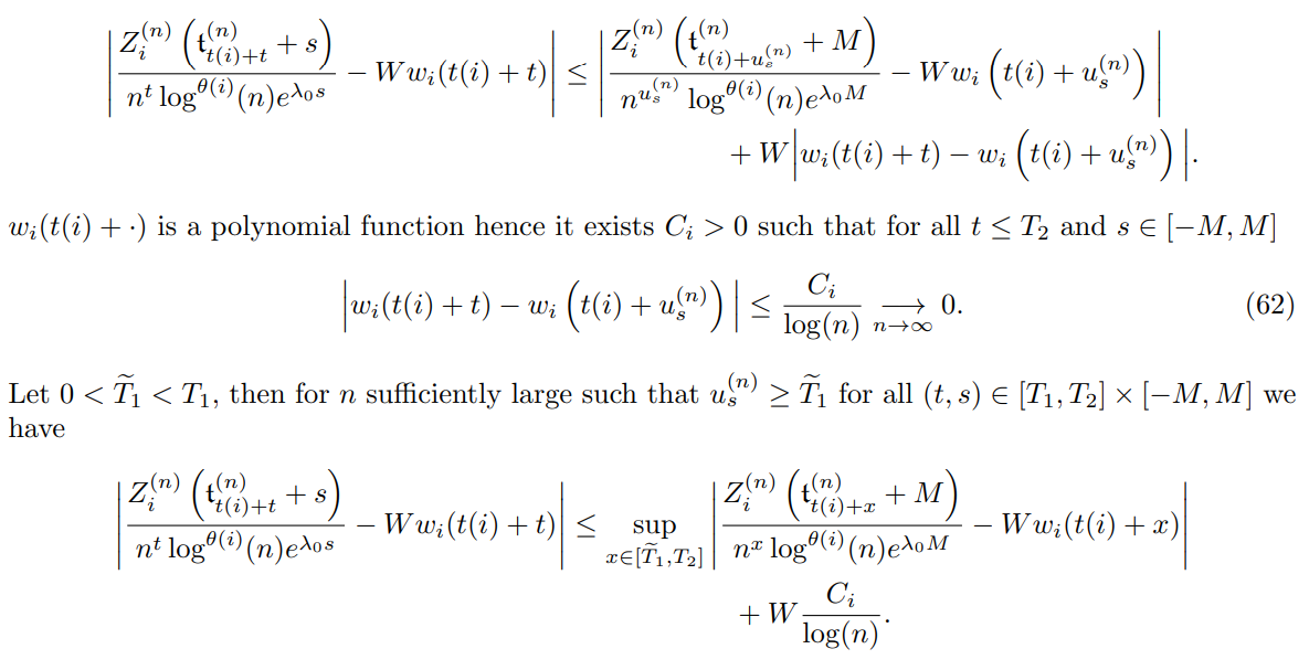
Hence we get for n sufficiently large
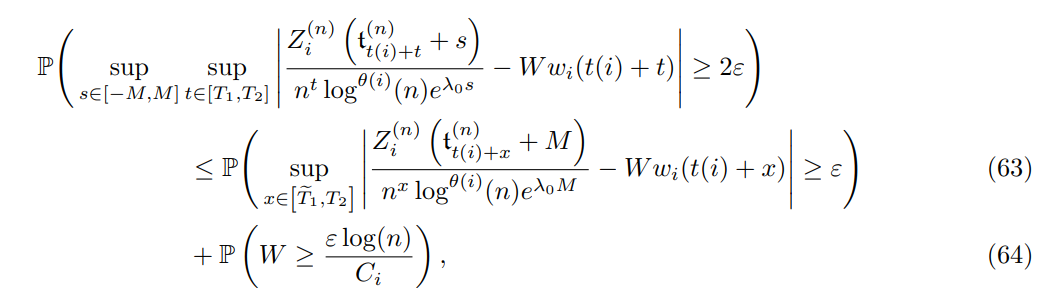
from which (12) is obtained. Indeed the term (63) converges to 0 according to Equation (28) and (64) converges to 0 since W is finite almost surely (see (20)).
We now show Equation (11). We have
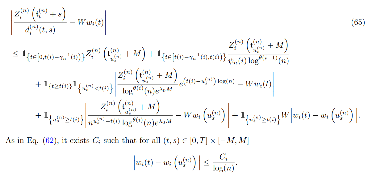

Finally using (65) and (66) we obtain for all (t, s) ∈ [0, T] × [−M, M]

Then it follows that

where the different convergences to 0 are obtained in the following way:

3.3 First-order asymptotics of the mutant sub-populations in the random time-scale (Theorem 2.1 (ii))