As we saw from the previous blog, the SIS algorithm is degenerate, which simply means that after some observations, relatively small in number, one of the particles achieves a weight close to 1. A solution has been proposed to sample the particles at each time observation.
SIR algorithm
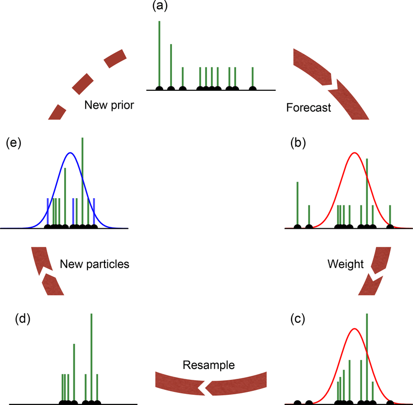
The SIR (sequential importance resampling) algorithm can be seen as a variant of SIS, but where at each time observation, we resample the paths from a simple multinomial distribution. This means that the particles with the highest weights will be resampled most often, hence we do not waste computational power in continuing the paths with negligible weights. This, however, introduces another problem, called particle impoverishment, which we shall focus on a bit later. The problem arises from the fact that since particles with large weights are likely to be drawn multiple times during resampling, whereas particles with small weights are not likely to be drawn at all, the diversity of the particles will tend to decrease after a resampling step. To illustrate what happens, we run the SIR algorithm with only 4 particles and plot them, while observing them being resampled:
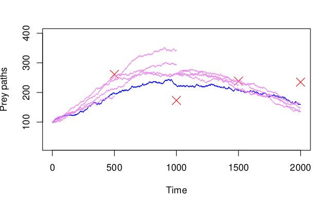
If we look at time 1000, we see that two of the paths have not been resampled at all, which means that while they have low weights, we start to lose diversity in the paths. What is more, it seems that we have collapsed onto a single path at time 1000 onwards, which leaves us with the same issue as with the SIS algorithm. Nevertheless, the algorithm is easy to code, and while it does lead to particle impoverishment, more often than not, it seems to perform within some desirable limits [1]. In most of the situations, the more or less “extreme” case shown in the figure above, is not as pronounced.
Filtering
We have already described the idea behind filtering at the beginning the last post, i.e. to try to guess the distribution of the state of the hidden process at the current time, given the data up to now. This can also be thought of a “tracking” problem, where we keep track of the location of the system noisy observations. One simple way of restoring the hidden path is by doing a weighted average with respected to the weights at each time interval. In particular, imagine that we have just received our j-1 noisy observation and we have resampled our particles. Then each of the particles will have a weight of 1/N and when we receive the j observation, the weights will correspondingly be \{w_{j}^{i}\}_{i=1}^{N}, for the particles \{\mathbf{x}_{j}^{i}\}_{i=1}^{N}. We can introduce the weight vector at time j as \mathbf{w}_{j} = (w_{j}^{1}, w_{j}^{2}, \ldots, w_{j}^{N}) and the corresponding particle trajectories in a matrix form as \mathbf{x}_{j} = ((\mathbf{x}_{j}^{1})^{T}, (\mathbf{x}_{j}^{2})^{T}, \ldots, (\mathbf{x}_{j}^{N})^{T}). Then we can perform a weighted average over every single time segment and connect the predicted paths over the segments. Hence, if we denote the approximated path as \mathbf{x}_{best}, it will take the form:
\mathbf{x}^{best} = (\mathbf{x}^{best}_{1}, \mathbf{x}^{best}_{2}, \ldots, \mathbf{x}^{best}_{j}),
where \mathbf{x}^{best}_{s} = \mathbf{x}_{s}\mathbf{w}_{s}^{T}, for all s \in \{1, \ldots, N\}. After performing the simulation, we achieve the following plot:

It is interesting to point out that the plot below was produced using 100 particles. Running the particle filter for 1000 particles instead introduces only a slight improvement, while considerably increasing the running time. In fact, on my computer the simulation took about 3 seconds for 100 particles and approximately 30 seconds for 1000 particles, suggesting an \mathcal{O}(n) complexity when it comes to the number of particles, which is further confirmed by [2].