Article

Antarctic Sea-Ice Thickness Retrieval from ICESat: Inter-Comparison of Different Approaches

1
Integrated Climate Data Center (ICDC), Center for Earth System Research and Sustainability (CEN), University of Hamburg, 20144 Hamburg, Germany
2
Polar Research Center (PolReC), Maritime Faculty, Istanbul Technical University (ITU), 34940 Istanbul, Turkey
3
Antarctic Climate and Ecosystems Climate Research Center (ACE CRC), University of Tasmania, 7000 Hobart, TAS, Australia
*
Author to whom correspondence should be addressed.
Remote Sens. 2016, 8(7), 538; https://doi.org/10.3390/rs8070538
Submission received: 30 March 2016 / Revised: 31 May 2016 / Accepted: 14 June 2016 / Published: 24 June 2016
(This article belongs to the Special Issue Sea Ice Remote Sensing and Analysis)

Abstract

:
Accurate circum-Antarctic sea-ice thickness is urgently required to better understand the different sea-ice cover evolution in both polar regions. Satellite radar and laser altimetry are currently the most promising tools for sea-ice thickness retrieval. We present qualitative inter-comparisons of winter and spring circum-Antarctic sea-ice thickness computed with different approaches from Ice Cloud and land Elevation Satellite (ICESat) laser altimeter total (sea ice plus snow) freeboard estimates. We find that approach A, which assumes total freeboard equals snow depth, and approach B, which uses empirical linear relationships between freeboard and thickness, provide the lowest sea-ice thickness and the smallest winter-to-spring increase in seasonal average modal and mean sea-ice thickness: A: 0.0 m and 0.04 m, B: 0.17 and 0.16 m, respectively. Approach C uses contemporary snow depth from satellite microwave radiometry, and we derive comparably large sea-ice thickness. Here we observe an unrealistically large winter-to-spring increase in seasonal average modal and mean sea-ice thickness of 0.68 m and 0.65 m, respectively, which we attribute to biases in the snow depth. We present a conceptually new approach D. It assumes that the two-layer system (sea ice, snow) can be represented by one layer. This layer has a modified density, which takes into account the influence of the snow on sea-ice buoyancy. With approach D we obtain thickness values and a winter-to-spring increase in average modal and mean sea-ice thickness of 0.17 m and 0.23 m, respectively, which lay between those of approaches B and C. We discuss retrieval uncertainty, systematic uncertainty sources, and the impact of grid resolution. We find that sea-ice thickness obtained with approaches C and D agrees best with independent sea-ice thickness information—if we take into account the potential bias of in situ and ship-based observations.

Graphical Abstract

1. Introduction

Antarctic sea ice plays a key role in the ocean-atmosphere heat, impulse, and matter exchange and is of profound importance for species as living and hatching ground. The Antarctic sea-ice cover is highly variable and—in contrast to its Arctic counterpart—does not yet show a decrease in its overall extent over the satellite era [1,2]. One of the key shortcoming in future climate scenario investigations as well as in the understanding of the inter-annual regional Antarctic sea-ice extent variability is given by the still widely unknown Antarctic sea-ice thickness distribution. The lack of this information has led to efforts to, for example, re-construct Antarctic sea-ice thickness distribution by means of numerical modeling (see e.g., [3]).
Sea-ice thickness information can be obtained most accurately by in situ measurements carried out during expeditions. However, only a limited amount of such measurements is available [4] and the vast majority of the sea-ice cover remains unsampled. What alternatives do exist? Ship-based visual observations carried out according to the Antarctic Sea Ice Processes and Climate (ASPeCt) protocol [5,6] are of limited spatio-temporal coverage as well, as illustrated by the track maps shown in [7]. Upward looking sonar (ULS) data are—in contrast to the Arctic—only available from moorings [8,9] and provide very useful temporal but quite limited spatial information about sea-ice thickness. Only recently, autonomous underwater vehicles (AUV) equipped with ULS devices allowed a first glimpse of Antarctic sea-ice thickness from below also over kilometer scales [10]. Satellite remote sensing is required to obtain a circum-Antarctic sea-ice thickness distribution.
Synergistic supervised classification and analysis of observations from various remote sensing sensors is used for so-called ice charts which provide, among sea-ice concentration, type and state of development, also information about the sea-ice thickness range. This information has been exploited by [11,12] who derived seasonal and annual estimates of the Antarctic sea-ice thickness and volume for 1995–1998. Satellite infrared temperature measurements can be used to obtain sea-ice thickness but only for thin ice regions [13,14]. Imaging satellites such as active and passive microwave sensors have also been used to retrieve Antarctic sea-ice thickness. The sea-ice thickness range within which these sensors provide useful information is, however, under debate and is a function of frequency, region, and season [14,15,16,17,18,19,20,21]. Passive microwave sensors measure the brightness temperature, which can be used to retrieve primarily the thickness of thin sea ice [14,15], i.e., sea ice thinner than ~0.2 m. This is sufficient to estimate ice production in Antarctic coastal polynyas [16]. The retrieval is based on the relationship between the microwave emissivity of the sea ice and its dielectric properties. These are primarily influenced by the sea-ice salinity which is a function of temperature and thickness of the sea ice. The salinity of thin and first-year sea ice is larger at the surface than in the deeper layers of the sea ice; the salinity profile has a C-shape. The salinity therefore influences the penetration depth of the microwave radiation into the sea ice. This limits sea-ice thickness retrieval using most passive microwave sensors to maximum ~0.2 m. The method of Aulicino et al. [18], which combines the microwave frequencies used by [14,15,16] in a different way, seems to succeed in retrieving larger sea-ice thickness values. However, this method is limited to values below 1 m and has only been tested for the southern Ross and Weddell Seas. Another alternative is given by the Soil Moisture and Ocean Salinity (SMOS) sensor. The SMOS sensor operates at L-band and its brightness temperatures are routinely used to retrieve sea-ice thickness up to ~0.7 m in the Arctic [19]; SMOS data are currently also being tested for Antarctic sea-ice thickness retrieval. Active microwave sensors measure the amount of microwave radiation emitted to and scattered back by the sea ice. Like is the case for brightness temperatures, the amount of radiation scattered back is a function of the salinity of the sea ice and therefore of its thickness. For Antarctic sea ice, only a few studies exist which have used active microwave data to estimate sea-ice thickness directly from radar backscatter e.g., [17]. The limited coverage of high-resolution synthetic aperture radar (SAR) images, which are required for this approach, is one of the main impediments. Other limitations are given by ambiguities in the radar backscatter signal. These two limitations are also valid for another, indirect method to retrieve sea-ice thickness from SAR imagery. This method exploits the fact that the wave spectrum of ocean swell entering the sea ice changes as a function of sea-ice thickness [20,21]. The main application area for this method is the pancake ice of the marginal ice zone. The thickness of sea ice into which swell does not penetrate cannot be retrieved with this method.
What remains is satellite altimetry. Two types of sensors exist: radar altimetry to estimate sea-ice freeboard—provided that the radar signal is reflected at the ice-snow interface—and laser altimetry to estimate total (sea ice + snow) freeboard. While radar altimetry has been successfully employed in the Arctic, e.g., Laxon et al. [22,23], difficulties arise in the Antarctic [24]. An unknown fraction of the radar signal is not reflected at the ice-snow interface but somewhere inside the snow layer or even at the snow surface [25]. Work to improve Antarctic sea-ice freeboard retrieval with radar altimetry is ongoing [26] but not part of the present study which focuses on laser altimetry.
For laser altimetry, snow properties are less of an issue for the retrieval of the total freeboard and therefore sea-ice thickness retrieval. By using data of the Geoscience Laser Altimeter System (GLAS) aboard the Ice, Cloud and land Elevation Satellite (ICESat) Antarctic sea-ice thickness has been estimated in various regions. Markus et al. [27] focused on East Antarctic sea ice, Xie et al. [28] focused on the Bellingshausen and Amundsen Seas, and Zwally et al. [29], Yi et al. [30] and Kern and Spreen [31] focused on the Weddell Sea. Kurtz and Markus [32] were the first to provide circum-Antarctic sea-ice thickness and volume estimates based on ICESat data. However, there is evidence that the main assumption made in [32]: sea-ice freeboard is zero everywhere and the elevation measured by ICESat equals snow depth, could have resulted in a considerable sea-ice thickness underestimation [31,33]. The main driver for that assumption was to avoid inclusion of snow-depth information into the sea-ice thickness retrieval. Snow depth on Antarctic sea ice is complex, difficult to obtain, and seems to be unbiased only when retrieved from satellite observations over undeformed seasonal sea ice (see e.g., [34]).
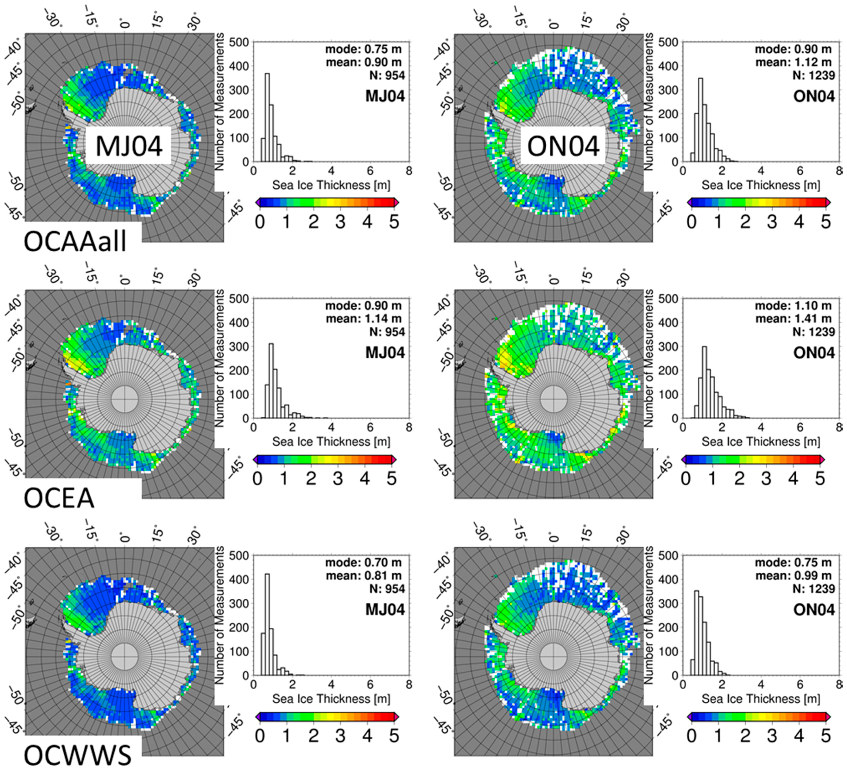
Motivated by these results we carry out a qualitative inter-comparison of sea-ice thickness retrieved from ICESat total freeboard using a number of different approaches—including the data of [32]. Except this data, all approaches presented in this paper are based on total freeboard retrieved from ICESat data following [31]. None of these assume that sea-ice freeboard is zero. Instead we apply different ways to treat snow depth on sea ice, e.g., a snow depth climatology, a modified sea-ice density, or different empirical approaches to directly convert total freeboard into sea-ice thickness. At first glance, we find that sea-ice thickness obtained with the empirical approaches seem to agree better with in situ and ship-based observations during winter and spring. However, if we take into account that the observations are potentially biased low, then the “classical” approach for Antarctic sea ice [29,30], named SICCI approach [31] here, and the approach utilizing a modified sea-ice density seem to perform best in comparison to the above-mentioned observations and other independent observations detailed in the paper.
We lay out the approaches in the following section after the description of the data. We present our results in Section 3 and we discuss these in Section 4, before we give some concluding remarks in Section 5.

2. Materials and Methods

2.1. Data

We use GLAS/ICESat L2 sea-ice altimetry data (GLA13) of release 33 altimetry binary [35]. The data are downloaded for ICESat measurement periods 2B to 3J from the U.S. National Snow and Ice Data Center (NSIDC) [35]. These data are used to compute the circum-Antarctic distribution of the total freeboard and sea-ice thickness as described in [31]. We compute maps of the total freeboard at 25 km and at 100 km grid resolution separately for each ICESat period from 2B (February/March 2004 or FM04) to 3J (February/March 2008 or FM08) (see Table 1).
Note that data need to be averaged over such long periods—about 33–35 days long—to obtain a sufficiently dense coverage with valid data. In addition maps of the freeboard retrieval uncertainty are computed as described in [31] and are used to derive sea-ice thickness retrieval uncertainty where applicable. We focus on the winter (MJ) and spring (ON) periods. We use the abbreviations given in Table 1 in parentheses if we refer to specific periods. Otherwise we refer to winter or spring. We also henceforth abbreviate May/June as MJ and October/November as ON.
We downloaded gridded total freeboard and sea-ice thickness published by [32] (see also [27]) from the Cryosphere Science Research Portal at NASA: http://seaice.gsfc.nasa.gov/csb/index.php?section=272). This data set contains total freeboard estimated with the approach described in [27] and sea-ice thickness (see Section 2.2 for details) on the NSIDC polar stereographic grid with tangential plane at 70°S with 25 km grid resolution.
For the approaches, which require snow depth data to convert total freeboard into sea-ice thickness (see Section 2.2), we use the AMSR-E snow depth data set [36]. This data comes daily as 5-day mean values for 2002 to September 2011. The data does not include any uncertainty information. We reprojected the snow depth data from 12.5 km NSIDC polar-stereographic grid with tangential plane at 70°S to the corresponding grid with 25 km and 100 km grid resolution for each ICESat measurement period (Table 1).
Sea-ice concentration data are required to limit the sea-ice thickness retrieval to the sea-ice covered area. All but the approach of [32] use the IFREMER-UHAM daily 5-day median-filtered ARTIST Sea Ice (ASI) algorithm sea-ice concentration data set: http://icdc.zmaw.de/1/daten/cryosphere/seaiceconcentration-asi-ssmi.html [37,38]. This data set has 12.5 km grid resolution, using the same polar-stereographic grid as the snow depth data set (see above). In the freeboard retrieval and also later in the freeboard-to-thickness conversion we only use grid cells with SIC > 60%. The AMSR-E snow depth data set (see above) as well as the product by [32] includes AMSR-E NASA-Team 2 algorithm SIC data at 12.5 km grid resolution [36].

2.2. Methods

This section gives an overview about the methods used to convert total freeboard to sea-ice thickness. The approaches listed in Section 2.2.1, Section 2.2.2, and Section 2.2.5 require at least an estimate of the sea-ice density if not also densities of sea water and snow. Unless stated otherwise we use the following densities [30]: Open water: ρ water = 1023.9 kg/m3, snow: ρ snow = 300.0 kg/m3, sea ice: ρ ice = 915.1 kg/m3. In order to investigate the sensitivity to sea-ice density we also ran the SICCI approach (see Section 2.2.1) with density values of 900.0 kg/m3 and 875 kg/m3, which are the values used by [32].

2.2.1. The SICCI Approach

As suggested by [29] and confirmed by [30] it seems to be practical to discriminate between positive sea-ice freeboard and negative sea-ice freeboard, i.e., potentially flooded sea ice. We take the difference total freeboard F minus snow depth S as criterion to decide whether sea-ice freeboard is positive or negative. If this difference is negative then the sea-ice freeboard is assumed to be negative. If this difference is positive then the sea-ice freeboard is assumed to be positive. To do so we assume that both F and S are accurately retrieved. The validity of this assumption is discussed in Section 4.
The SICCI approach [31] follows the methods proposed by [29,30] and computes sea-ice thickness I from F and S via Equation (1) if S < F, or via Equation (2) if S ≥ F. Note that Equation (2) is independent of S. It is obtained from Equation (1) by setting S = F [30]. Here it is assumed that the sea-ice freeboard is zero, that F equals the snow depth above the sea surface, and that any snow on the sea ice below the sea surface is flooded and can therefore be regarded as slush which has a similar density as sea ice (e.g., [39]).
F > S : I = F ρ water ρ water ρ ice S ρ water ρ snow ρ water ρ ice
F S : I = F ρ snow ρ water ρ ice
Total freeboard values > 1 m are discarded following [30]. Equations (1) and (2) are applied to gridded freeboard data at 25 km and 100 km grid resolution.
Sea-ice thickness retrieval uncertainties are computed using Gaussian Error propagation [31,40] applied to Equations (1) and (2) resulting in Equations (3) and (4):
F > S :   σ I 2 = ( dF ρ water ρ water ρ ice ) 2 + ( dS ρ snow ρ water ρ water ρ ice ) 2 + ( dρ snow S ρ water ρ ice ) 2 + ( dρ ice ρ water   F + ρ snow   S ρ water   S ( ρ water ρ ice ) 2 ) 2
F S :   σ I 2 = ( dF ρ water ρ water ρ ice ) 2 + ( dρ snow F ρ water ρ ice ) 2 + ( dρ ice ρ water   F ( ρ water ρ ice ) 2 ) 2
The contribution of the uncertainty in water density is considered small compared to the contributions of the other parameters. We neglect it therefore. As uncertainties for snow and sea ice density we use dρ snow = 50 kg/m3 and dρ ice = 20 kg/m3 (see [41]). As uncertainty of the snow depth we use dS = 0.3 × S. This is a rather conservative estimate—particularly when considering 100 km grid resolution data. However, snow depth products from satellite microwave radiometry like the one used are potentially biased low over deformed sea ice (see e.g., [42]) and for wet snow (e.g., [43]) but could be also biased high for coarse-grained snow [43]. These products lack uncertainty information. Both motivated us to choose such a conservative snow-depth uncertainty (see also [31]). As uncertainty for freeboard we use dF = 3 × dF’, dF’ = freeboard retrieval uncertainty. The motivation for multiplying the freeboard retrieval uncertainty with a factor of 3 is given and discussed in [31].
We chose relatively large values as input uncertainties to our error computation. We did so to mitigate the impact of an important shortcoming in our uncertainty computation. Ideally we should discriminate between random uncertainties—for which Gaussian Error propagation is the valid approach—and systematic uncertainties. A random uncertainty would be, for instance, the contribution of sensor noise to the brightness temperatures used to compute the snow depth from satellite microwave radiometry. A systematic uncertainty would be, for instance, the bias in snow depth for deformed sea ice. A separation of random and systematic uncertainties requires sufficient knowledge of both contributions, which is, however, not yet achievable to our best knowledge. Snow depth retrieved from satellite microwave radiometry is one example. Biases can exist both ways, as mentioned in the previous paragraph, and depend on environmental conditions with unknown spatio-temporal distribution. Freeboard retrieved from ICESat is another example. Total freeboard from SICCI could be biased high compared to the method used in the KandM data set (see Section 2.2.2) but this bias cannot be quantified without additional measurements. Locations where the geoid is biased, where anomalies in the mean sea surface height are not accounted for in the freeboard pre-processing, or where ocean swell influences ICESat elevation measurements are yet unknown and can bias total freeboard both ways. Therefore, we suggest to treat all uncertainty contributions as random, and we note that the obtained uncertainties are not just a measure of the random uncertainty (precision) but contain also information about the accuracy (potential bias).
In the following, we refer to this approach as “SICCI” because it has been developed as part the European Space Agency Climate Change Initiative Sea Ice project.

2.2.2. The Kurtz and Markus (KandM) Data Set

The approach of Kurtz and Markus [32] differs in several ways from the SICCI approach and from [29,30]. First the freeboard retrieval is different from the SICCI one. The SICCI approach employs a modified version of the lowest-level elevation method to obtain tie points of the sea-surface height in 50 km long segments centered at each laser shot along the ICESat track (see [29,30,31]). The KandM approach employs a linear relationship between the 25 km scale along-track ICESat surface roughness and the along-track ICESat surface elevations of leads identified in near-coincident spaceborne visible imagery taken from the entire Southern Ocean for spring 2003 and winter 2005 to obtain tie points of the SSH [27]. This relationship is applied to each laser shot. The freeboard retrieval after [27,32] results in slightly smaller overall mean total freeboard than the SICCI approach; for the Weddell Sea the difference is 0.06 m when averaged over all 9 ICESat measurement periods for years 2004 to 2006 [31]. For the entire Antarctic we find modal values of the difference in total freeboard between 0.05 to 0.1 m for basically all periods investigated (see also Section 4.2). Secondly, the freeboard-to-thickness conversion assumes zero sea-ice freeboard everywhere [32]. This way the discrimination between positive and negative sea-ice freeboard based on satellite-based snow depth, which is required by the SICCI approach, is avoided which could be an advantage. As another advantage, setting the sea-ice freeboard to zero implies that the measured total freeboard equals the snow depth. Hence a separate snow depth data set is not required to convert freeboard to thickness. Third, values of sea-ice density and snow density are chosen to vary seasonally. For winter and spring, sea-ice density is 900 kg/m3 and for fall the value chosen is 875 kg/m3. Snow densities are 320 kg/m3, 350 kg/m3, and 340 kg/m3 for spring, fall, and winter, respectively [32]. In the following, we refer to this approach as “KandM”.

2.2.3. Empirical Approaches from in Situ Measurements (OC2013)

By using in situ observations of sea-ice thickness, snow depth and freeboard from 15 research cruises into the Southern Ocean Ozsoy-Cicek et al. [4] proposed a suite of regional empirical approaches which allow direct conversion of total freeboard into sea-ice thickness without including snow depth and density information.
We test these approaches as follows: [4] derived empirical relationships, i.e., a set of linear regression coefficients, for five different regions in the Southern Ocean: Western Weddell Sea (WWS), Eastern Weddell Sea, Eastern Antarctic (EA), Ross Sea, and Bellingshausen-Amundsen Sea. From these relationships we pick two: WWS and EA because for WWS the relationship can be expected to be dominated by perennial sea ice and because both regions, WWS and EA (see Figure 1, right), showed the most extreme values of the five regions investigated. In addition to these two sets of regression coefficients, we compute an overall Antarctic (AAall) set of regression coefficients. These three sets are given together with uncertainty estimates of the coefficients (see [4]) in Table 2.
Based on these regressions sea-ice thickness I and its uncertainty σ I are computed (in meters):
I = 0.01   ( b + a   F )
σ I = 0.01   ( a   dF ) 2 + ( F   da ) 2 + ( db ) 2
In the following, we refer to this approach as “OC2013” when talking about this approach in general and as “OCAAall”, “OCEA”, and “OCWWS” for the specific approaches.

2.2.4. SICCI Approach Using SSM/I Snow-Depth Climatology (MandC)

Instead of using daily—or in our case—monthly varying snow-depth data of perhaps inferior quality and representativity one could use a snow-depth climatology. Instead of using inter-annually varying monthly mean AMSR-E snow depths to compute the sea-ice thickness from the SICCI freeboard estimates with Equations (1) and (2) we use the mean circum-Antarctic snow-depth climatology given in [43]. The respective snow-depth values are based on Special Sensor Microwave/Imager data: 23 cm for fall and 13 cm for both winter and spring, and are kept constant for every grid cell and every year. We note that this is a very simple way of using snow depth in the freeboard-to-thickness conversion. All other parameters except the snow depth are the same as described in Section 2.2.1. In the following, we refer to this approach as “MandC”.

2.2.5. Replacing Snow Depth with Modified Sea-Ice Density (Worby)

Another approach to get rid of the problem of a potentially biased snow depth from satellite microwave radiometry would be to completely omit usage of snow-depth data—as is also done in the KandM (Section 2.2.2) and OC2013 (Section 2.2.3) approaches—and instead treat the sea ice-snow system as one layer with reduced density. Here we assume that the density of the one-layer sea ice-snow system changes linearly with the ratio sea-ice thickness to snow depth. We note that this assumption requires that the sea ice with its snow cover is in isostatic balance following Archimedes’ principle. This is the assumption which is used in all approaches applied in this paper. For a unit (1 m2) area we can then write for a volume of sea ice plus snow:
( I + S ) ρ ice * = I ρ ice + S ρ snow
This equation can be solved for ρ i c e * and, by using R = I S , written as:
ρ ice * = R   ρ ice + ρ snow R + 1
with R being a seasonally dependent factor. For the present paper, we compute R from ASPeCt sea-ice thickness and ASPeCt snow depth observations. Following [6] the mean circum-Antarctic fall, winter and spring average sea-ice thickness I is 0.68 m, 0.66 m and 0.81 m, respectively. These values include contributions from ridged ice which we believe is the right set of values to be used for ICESat which measures ridged ice as well. The respective mean circum-Antarctic snow depth S is 0.10 m, 0.11 m, and 0.15 m, respectively. This results in R values of 6.8, 6.0, and 5.4 for fall, winter, and spring, respectively. These translate into apparent sea-ice densities ρ ice * of: 836 kg/m3, 827 kg/m3, and 819 kg/m3. Note that these are not the “real” sea-ice densities as are used by [32], see Section 2.2.2, but the density of a layer which incorporates the snow layer on top.
We note that R—as we use it in this paper—does not take into account the small-scale or even regional variability of the snow depth on sea ice. None of the approaches shown in the present paper can take into account small-scale variations—neither in sea-ice thickness and density nor in snow depth and density—beyond those which are resolved by the ICESat freeboard measurements. In Section 4 we will show how R, ρ ice * , and sea-ice thickness change as function of regional ASPeCt observations of sea-ice thickness and snow depth.
We compute the sea-ice thickness then via:
I = F   ρ water ρ water ρ ice *
In order to evaluate whether Equations (8) and (9) provide reasonable estimates of the sea-ice thickness we computed R, ρ ice * , and the sea-ice thickness for in situ measurements of the following Antarctic expeditions: GLOBEC in 2002 [44], ARISE in 2003 [45], ISPOL in 2004 [46], SIMBA in 2007 [47] and SIPEX-I in 2007 [48]. The majority of the in situ measurements carried out during these cruises took place in September/October. We find an average observed sea-ice thickness from N = 46 in situ measurement profiles of 1.13 m ± 0.51 m. About two thirds of the observations fall into the sea-ice thickness bins 0.5 to 1.0 m (17 profiles) and 1.0 to 1.5 m (15 profiles). We compute sea-ice thickness obtained with Equation (9) using the observed total freeboard, a water density of ρ water = 1023.9 kg/m3 and values of ρ ice * , which we computed using Equation (8) for a sea-ice density of 900 kg/m3 and a snow density of 300 kg/m3, and we find an average sea-ice thickness based on the Worby approach of 1.21 m ± 0.59 m. The average difference between observed and computed sea-ice thickness is 0.08 m, the RMSD of the sea-ice thickness values is 0.23 m. Observed sea-ice thickness values range between 0.22 m (computed: 0.22 m) and 2.41 m (computed: 2.64 m). The average R value of 44 profiles is 5.1 ± 2.2 with a minimum of 1.6 and a maximum of 11.5. We excluded two even more extreme values of 17.8 and 57.5 from the computation of the average R value. These extremes belong to medium thick sea ice (0.89 m and 1.15 m) with a very thin snow cover (0.05 m and 0.02 m) for which we obtain sea-ice thickness values of 0.72 m and 0.84 m, respectively, using Equation (9).
In the following, we refer to this approach as “Worby”.

2.2.6. Choice of the Grid Resolution

It has been demonstrated by Weissling and Ackley [49] that to properly represent the statistical properties of the Antarctic sea-ice thickness distribution with ICESat, ICESat measurements over a length scale of about 15 to 20 km are required. This agrees well with the 25 km along-track length scales used in the various approaches to retrieve Antarctic sea-ice thickness [27,28,29,30,32]. The primary goal of the SICCI project is to generate a gridded sea-ice thickness product—such as the one of [32]. As is demonstrated in [31], a grid resolution of 25 km provides a very sparse coverage with ICESat data. Many grid cells do not contain any data. In the majority of the grid cells, ICESat data from basically 1–2 days within the 33- to 35-day ICESat measurement periods (Table 1) can be used to derive a gridded sea-ice thickness value. The reason for the sparse data coverage is on the one hand the limited number of satellite overpasses per grid cell. On the other hand filtering of the data, in particular for attenuation by clouds in the atmosphere, causes a substantial amount of data being discarded. Figure 1 exemplifies the data coverage at 25 km grid resolution by showing the total freeboard obtained with SICCI for an ICESat period with good data coverage (MJ05) and a period with poor data coverage (ON06).
Using 100 km grid resolution allows assigning a larger fraction of the sea-ice cover with a sea-ice thickness estimate. In addition, the average number of days from which ICESat data contribute to a grid cell value increases from 1–2 days to 3–4 days. The average number of single shot values used per grid cell increases from ~100 at 25 km grid resolution to ~1000 at 100 km grid resolution. However, as a disadvantage at 100 km grid resolution, potentially erroneous freeboard estimates and therefore sea-ice thickness values could be amplified because they are assumed to represent an area of 100 km × 100 km. Another disadvantage is that it is more difficult to estimate the modal sea-ice thickness at coarser grid resolution, particularly for fall, when only few grid cells contain valid sea-ice thickness values. Finally, because of the asymmetric shape of the sea-ice thickness distribution modal and mean sea-ice thickness values derived for the entire Southern Ocean could differ between 100 km and 25 km grid resolution.
However, the main goal of this paper is to qualitatively inter-compare different freeboard-to-thickness conversion approaches applied to the same freeboard data set. Table 3 shows that the differences in modal and mean circum-Antarctic total freeboard between 100 km and 25 km grid resolution are <2 cm for winter (MJ) and spring (ON).

3. Results

The SICCI (Section 2.2.1) sea-ice thickness and the KandM (Section 2.2.2) sea-ice thickness issued by [32] are the only freely available circum-Antarctic sea-ice thickness products. Therefore we present the results of their inter-comparison first (Section 3.1). Note that these two approaches were compared already in [31] but only for the Weddell Sea region. In Section 3.2 we inter-compare the results of SICCI with the results obtained by applying the other approaches described in Section 2.2.3, Section 2.2.4 and Section 2.2.5 to the same total freeboard data as SICCI.

3.1. Inter-Comparison of SICCI versus KandM Sea-Ice Thickness

Figure 2 illustrates that in winter new ice formation has advanced around all of the Antarctic providing a wide belt of sea ice with a thickness of 0.5 to 1.5 m. The most extensive zones of such thin sea ice are found in the central Weddell Sea and in most of the Ross and Amundsen Seas. Thicker sea ice is found along the East Antarctic coast, in some coastal areas in the Amundsen Sea, and in the Weddell Sea. The latter is known for a substantial amount of perennial sea ice hugging the Antarctic Peninsula—as is demonstrated by the SICCI sea-ice thickness map (see also [29,30,31]). From winter to spring the amount of thicker sea ice increases while thin sea ice with values <1 m stays mainly in the central Weddell Sea. In addition, in the southern Ross Sea where the area downstream of the Ross Ice Shelf polynya is known to be covered by thin sea ice shows thickness values <1 m. The sea-ice thickness distribution in the Weddell Sea agrees well with the results of [30].
The KandM sea-ice thickness distribution tends to show similar features but the differences between the presumably perennial sea ice and seasonal sea ice are much smaller. In particular, sea-ice thickness >2 m is practically absent in contrast to SICCI results. KandM sea-ice thickness histograms do not reveal a tail towards high sea-ice thickness for winter or spring.
Both approaches reveal areas of spuriously high sea-ice thickness close to the ice edge, e.g., in MJ04 in the northeastern Weddell Sea or in ON04 in the northeastern Ross Sea. For SICCI these are examples where the coarse grid resolution amplifies erroneously high sea-ice thickness in areas with low data density (see discussion in Section 2.2.6). KandM sea-ice thickness data originally have a finer grid resolution: 25 km, but a kriging interpolation with a search radius of 125 km is used to interpolate between ICESat overpasses. SICCI does not interpolate between overpasses (see also Section 4.2). Maps obtained with both methods (KandM and SICCI) show these features. We therefore conclude that these are not caused by the differences in sea surface height approximation of the two methods, but instead suggest that the spuriously high sea-ice thickness is rooted in the freeboard retrieval in general. For instance, ocean swell can penetrate the sea-ice cover for several hundreds of kilometers. Undulations of the sea and sea-ice surface caused by swell could be misinterpreted by ICESat as elevated freeboard values. These could very likely explain spuriously high sea-ice thickness values along the ice edge. It seems to be less likely that an increase in total freeboard due to locally intense snow fall and/or due to locally elevated sea-ice freeboard caused by ice deformation processes such as rafting of thin sea ice has caused the high sea-ice thickness right at the ice edge. An incorrect geoid or mean sea surface model can also potentially cause erroneous total freeboard values, as has been shown for the Arctic by, e.g., [50].
We computed the difference SICCI minus KandM sea-ice thickness. We show the resulting maps and histograms for winter and spring in Figure 3 and Figure 4, respectively. The maps illustrate that SICCI over-estimates sea-ice thickness compared to KandM for most of the sea-ice cover. In only a few areas the difference SICCI minus KandM sea-ice thickness is below ±0.4 m; note that 0.4 m corresponds to the modal SICCI sea-ice thickness uncertainty at 100 km grid resolution (see also Section 4.1). In 2004, these areas are located in the central to western Weddell Sea and in the northern Ross and Amundsen Seas. The location of these areas changes from year to year (Figure 3). We summarize the seasonal average values of the modal and mean difference SICCI minus KandM sea-ice thickness in Table 4.

3.2. Inter-Comparison of SICCI versus OC2013, MandC, and Worby Sea-Ice Thickness

For winter (Figure 5) SICCI (Section 2.2.1) and Worby (Section 2.2.5, one-layer) are most similar in the spatial sea-ice thickness distribution on the maps as well as in the histograms. SICCI has more thin ice in the Weddell and Ross/Amundsen Seas than Worby. The thickest ice found in the western Weddell Sea hugs the Antarctic Peninsula more closely in SICCI than in Worby, where thicker ice extends a bit further to the East. Sea-ice thickness in the Eastern Antarctic seems quite similar between the two approaches. This good agreement also occurs in years 2005 and 2006 so that the average winter (2004–2006) mean sea-ice thickness agrees within 0.05 m between these two approaches (Table 5). The MandC (Section 2.2.4, climatological snow depth) sea-ice thickness distribution is more similar to Worby than to SICCI, however, gradients in the sea-ice thickness distribution are more pronounced. Where Worby shows thin sea ice MandC tends to show even thinner sea ice (Weddell and Ross Seas) and where Worby shows thick sea ice MandC shows even thicker sea ice. The latter applies especially to the western Weddell Sea where MandC shows a large area with sea-ice thickness >4 m. MandC modal sea-ice thickness is similar to SICCI and Worby, and the tail towards thicker sea ice is more pronounced. This is also valid for 2005 and 2006 (not shown). MandC has the largest average winter mean sea-ice thickness: 1.68 m of the four approaches compared in Figure 5. The OC2013 (Section 2.2.3, empirical; here OCAAall, see Table 2) sea-ice thickness distribution has smaller sea-ice thickness gradients and particularly has thinner sea ice along the Antarctic peninsula. The modal sea-ice thickness is 0.7 m and hence 0.2 m below the modal sea-ice thickness of the other three approaches compared in Figure 5 (see Table 5). Sea ice thicker than 2 m is practically absent as the histogram quickly tails to zero at sea-ice thickness ~2 m. This is the same for 2005 and 2006 (not shown). In that respect OCAAall is quite similar to KandM (Figure 2, Table 4).
For spring (Figure 6) the most pronounced change in the sea-ice thickness distribution of all approaches is an increase in sea-ice thickness and in the amount of thick sea ice. Modal and mean sea-ice thickness increase. The largest shifts in the histograms occur for SICCI and MandC (Section 2.2.4, climatological snow depth). For all but OCAAall (Section 2.2.3, empirical) most regions with sea-ice thickness between 0 and 1 m (1 and 2 m) in winter (Figure 5) exhibit sea-ice thickness between 1 and 2 m (2 and 3 m) in spring (Figure 6). The number of grid cells with sea ice thicker than 3 m has also increased. Common to all approaches is the thin sea-ice thickness of 1–2 m in the Ross Sea downstream of the Ross Ice Shelf polynya. MandC has by far more thick sea ice than Worby (Section 2.2.5, one-layer) and is more similar to SICCI than Worby is. The main difference between MandC and Worby on the one hand and SICCI on the other hand is a large region of sea ice thinner than 1 m in the SICCI model in the central Weddell Sea; this is different in years 2005 and 2006 (not shown). OCAAall sea-ice thickness is considerably smaller. Sea-ice thickness >2 m is almost absent in the OCAAall product—similar to KandM (Figure 2 and Figure 6).
Figure 7 illustrates the differences between OCAAall and OCEA, which is based on regression results of in situ measurements of sea ice in region East Antarctic, and OCWWS, which is based on regression results of in situ measurements of sea ice in region Western Weddell Sea (see also Figure 1, right). While the latter region comprises a substantial fraction of perennial ice, the former comprises measurements primarly on seasonal ice [4]. Both regions had less than three profiles with negative sea-ice freeboard due to flooding and exhibit the two largest mean sea-ice freeboard heights of the five regions investigated by [4]: 3.6 cm (OCWWS) and 4.7 cm (OCEA). Note that OCWWS is based on a very small number of profiles, though: 8 compared to OCEA: 22.
For winter (left column) sea-ice thickness distributions and histograms obtained with OCAAall and OCWWS look almost identical while OCEA shows more thick sea ice in the western Weddell Sea and the eastern Ross/Amundsen Seas. OCWWS results in the lowest mean sea-ice thickness of 0.81 m while OCEA provides the largest: 1.14 m. Only OCEA provides a significant fraction of grid cells with sea-ice thickness >2 m in the area covered by perennial sea ice along the Antarctic Peninsula. For spring (right column) the order is similar to winter. Sea-ice thickness >2 m is still practically absent for OCAAall and OCWWS and occupies a small but recognizable fraction for OCEA. These results are not surprising given the magnitude of the regression coefficients (Table 2). The interesting point is that these regressions, which are based on in situ measurements, provide (i) quite a small sea-ice thickness for winter and spring compared to the other approaches tested (Figure 5 and Figure 6) and provide (ii) results which can differ substantially depending on the set of regression coefficients used (compare OCWWS with OCEA in Figure 7).
Averaged over all three winters (Table 5), the largest modal sea-ice thickness is provided by MandC (Section 2.2.4 climatological snow depth) and Worby (Section 2.2.5, one-layer), followed by OCEA (Section 2.2.3, empirical) and SICCI. With regard to the mean sea-ice thickness, the order is MandC, SICCI, Worby, and OCEA. By far the smallest modal and mean values are provided by KandM (Section 2.2.2, zero sea-ice freeboard). Averaged over all four springs (Table 5), the largest modal sea-ice thickness is provided by SICCI followed by MandC, WORBY, and OCEA. With regard to mean sea-ice thickness the order is MandC, SICCI, Worby, and OCEA. Again KandM provides by far the smallest values.
How does the average mean sea-ice thickness change from winter to spring? Two classes of approaches can be identified. One class shows a large increase in sea-ice thickness: SICCI: 0.63 m and MandC: 0.50 m. The second class shows a moderate increase in sea-ice thickness: Worby: 0.23 m, OCEA: 0.20 m (0.16 m and 0.15 m for the other two OC2013 approaches). The average KandM sea-ice thickness increases only by 0.04 m. For the seasonal increase in average modal sea-ice thickness again two classes of approaches can be identified. One comprises MandC, OCEA, OCAAall, and Worby with an increase of the order of 0.2 to 0.3 m. The other comprises all other approaches—except SICCI—showing increases of the order of 0.10 m or less. SICCI stands out with an increase of 0.68 m.

4. Discussion

4.1. Retrieval Uncertainties

For SICCI (Section 2.2.1) and OCAAall (Section 2.2.3, empirical) we computed sea-ice thickness uncertainty estimates according to the equations provided in Section 2.2. Figure 8 shows sample uncertainty maps for SICCI for MJ04 and ON04.
The sample sea-ice thickness retrieval uncertainty maps and corresponding histograms shown in Figure 8 reveal: (i) the input parameters allow an estimation of the uncertainty for every grid cell; (ii) uncertainties stay within reasonable bounds with modal values of 0.3 to 0.5 m, mean values are slightly larger; (iii) uncertainties level off at ~1 m; (iv) largest uncertainties occur in areas of largest sea-ice thickness and hence presumably also deepest snow. We summarize the multi-annual seasonal average uncertainties in Table 6 for SICCI and OCAAall (Section 2.2.3, empirical). Retrieval uncertainties are larger in spring (ON) than in winter (MJ). Mean uncertainties are ~0.1 m larger than modal ones. Uncertainties for OCAAall are smaller than those for SICCI. Note, however, that for OCAAall, uncertainties are solely based on freeboard uncertainties and an estimated rather than computed uncertainty of the regression coefficients. In contrast, uncertainties for SICCI are based on the full set of uncertainties of all input parameters: freeboard, snow depth, densities. The uncertainties for SICCI should be taken as rather conservative values which include a considerable contribution by systematic errors (see Section 2.2.1)
We also estimated the retrieval uncertainty of the SICCI approach at a grid resolution of 25 km instead of 100 km. The multi-annual average modal uncertainty values shown in Table 6 for 100 km grid resolution increase by 0.09 m for winter and by 0.15 m for spring. The average mean uncertainties shown in Table 6 increase by 0.12 m and 0.13 m for winter and spring, respectively. This increase in the sea-ice thickness uncertainty is caused by the larger uncertainty of the gridded freeboard.
By taking the uncertainty values shown in Table 6 we find that for winter the multi-annual average modal SICCI sea-ice thickness agrees within its uncertainty bounds with all other approaches except KandM (Section 2.2.2, zero sea-ice freeboard). For the mean sea-ice thickness such agreement is only found with MandC (Section 2.2.4, climatological snow depth), Worby (Section 2.2.5, one-layer), and OCEA (Section 2.2.3, empirical). For spring (ON), the multi-annual average modal (mean) SICCI sea-ice thickness agrees within its uncertainty bounds only with MandC and Worby (only with MandC) (compare Table 5 and Table 6). We take this as an indication that the SICCI approach seems to provide reasonable sea-ice thickness values for winter, while for spring it is likely that SICCI over-estimates the sea-ice thickness. This could be caused by too small snow depths as will be discussed in Section 4.3.

4.2. Potential Biases Due to Freeboard Retrieval

Except KandM (Section 2.2.2, zero sea-ice freeboard), all approaches inter-compared in the present paper are based on total freeboard computed from ICESat using the approach of [31] which is a further development of [29,30]. For the Weddell Sea, gridded average modal total freeboard derived by [32] is 0.03 to 0.06 m and 0.05 to 0.11 m smaller than the one obtained by [31] for winter and spring, respectively ([31], Table 4); the differences in average mean total freeboard are similar. Here we extend this inter-comparison to the entire Antarctic.
Figure 9 shows two kinds of histograms for KandM. The full bars in the background denote the freeboard distributions using all grid cells of the KandM freeboard product while the open bars denote the grid cells co-located with SICCI freeboard. Note that [32] used kriging interpolation with a search radius of up to 125 km to interpolate gaps between single ICESat overpasses. In contrast, the SICCI approach [31] does not interpolate these gaps. All histograms illustrate the increase in freeboard from winter to spring. Shapes of the SICCI histograms and the co-located KandM histograms are relatively similar and confirm the results of [31]: SICCI provides slightly higher modal and mean total freeboard values. Co-located KandM freeboard distributions seem to be cut off at small total freeboard at bin 6–8 cm or 8–10 cm. The same distributions also seem to be cut-off at high total freeboard in spring between about 0.6 and 0.7 m. In contrast SICCI freeboard values tail off smoothly towards both ends of the histograms. It is very likely that the difference in total freeboard between SICCI and KandM is caused by the different ways with which the sea surface height tie points are obtained (see Section 2.2.2). A concluding inter-comparison between total freeboard derived with SICCI and with KandM would require independent observations of total freeboard from, e.g., air-borne sensors like in the Arctic [51]. To the authors’ best knowledge such air-borne observations being contemporary to ICESat ground tracks have not been carried out for Antarctic sea ice. Taking also into account the results of [28], who comment on the limitations of the approach of [29], and the recent work of [52], who discuss the limitations of ICESat in comparison to ICESat-2 to be launched in 2018, we cannot exclude that the circum-Antarctic SICCI total freeboard has an overall positive bias of a few centimeters. This could introduce a positive bias in the circum-Antarctic average modal and mean sea-ice thickness of between 0.2 and 0.6 m.
In Table 3 we showed that average modal and mean freeboard values obtained at 100 km grid resolution differ by less than 2 cm from those derived at 25 km for the winter and spring periods listed in Table 1. How does this difference translate into the sea-ice thickness computed from these freeboard data? To answer this question, we computed sea-ice thickness at 100 km and at 25 km grid resolution with the SICCI (Section 2.2.1) and the Worby (Section 2.2.5, one-layer) approaches. For SICCI, we find a decrease of the multi-annual average modal sea-ice thickness from 100 km to 25 km grid resolution by 0.12 m and 0.05 m for winter and spring, respectively. We find a smaller decrease of the respective mean sea-ice thickness values of 0.08 m for winter and 0.01 m for spring. For Worby, we find a decrease in modal sea-ice thickness by 0.07 m for winter but an increase by 0.04 m for spring while the mean sea-ice thickness decreases by 0.03 m for winter and remains unchanged for spring. We can attribute the larger changes in modal sea-ice thickness for winter to a reduction of the modal sea-ice thickness by 0.4 m (SICCI) and 0.2 m (Worby) for period MJ05.
These results illustrate two things. First, with 100 km grid resolution we are at the limit of obtaining a meaningful, representative circum-Antarctic sea-ice thickness distribution from ICESat data. As has been detailed in various recent studies about estimation of large-scale sea-ice thickness (e.g., [12]) and about spatial aliasing of sea-ice thickness measurements (e.g., [53]), any gridded sea-ice thickness products have to be used and interpreted with attention to the measurement scales involved. At 25 km grid resolution one would obtain a sea-ice thickness distribution which is perhaps more realistic but which still does not reflect the true sea-ice thickness distribution. Secondly, both approaches, also the conceptually new Worby approach, provide a robust estimate of the average seasonal circum-Antarctic sea-ice thickness. The differences obtained between 100 km and 25 km grid resolution are smaller than systematic uncertainties due to biases in freeboard or sea-ice density and much smaller than our conservative sea-ice thickness retrieval uncertainty estimates.

4.3. Potential Biases Due to Inaccurate Snow Depth

For the SICCI approach (Section 2.2.1), the discrimination of negative from positive sea-ice freeboard assumes that total freeboard F and snow depth S are accurately retrieved. For F it is unlikely that processes at the ice-snow interface influence the accuracy. For S, however, flooding may influence the accuracy substantially. Flooding increases snow basal layer wetness and salinity. Eventually the water is wicked further up into the snow. This could lead to a considerably negative bias in snow depth because of the changing snow dielectric properties in response to an increase in snow wetness [43]. The potential changes in the centimeter-scale surface roughness caused by subsequent re-freezing of the slush layer could also have an influence on the accuracy of S. However, it can be expected that this influence is smaller than that of increased snow wetness [43]. Therefore, in flooded areas retrieved snow depth might underestimate actual snow depth. Consequently, using the difference F minus S to identify negative sea-ice freeboard could result in fewer grid cells with negative sea-ice freeboard than are actually present. This would result in a larger number of grid cells where Equation (1) is used despite Equation (2) should be used. However, more importantly, using Equation (1) with an underestimated snow depth results in an overestimation of the sea-ice thickness.
Snow depth retrieved from satellite microwave radiometry is underestimated for deformed sea ice (e.g., [27,42,54]). Therefore, not only in areas with increased snow wetness but also in regions with deformed sea ice the snow depth used by SICCI is potentially underestimated, causing an overestimation of the sea-ice thickness.
The climatological snow depth used in the approach MandC (Section 2.2.4) is based on the snow depth computed from satellite microwave radiometry [43]. Therefore, in regions subject to frequent flooding and sea-ice deformation the snow depth climatology derived by [43] is likely to be biased low. This can cause an overall positive bias in the sea-ice thickness obtained with the MandC approach in addition to those sea-ice regions where the climatological snow depth underestimates the actual snow depth.
Snow ages and modifies under the action of heat and moisture fluxes through the ice-snow system which vary with the net radiation flux at the snow surface and with weather conditions such as wind speed, air temperature and humidity, and precipitation. As a consequence snow grain sizes increase.This occurs particularly during melt-refreeze cycles associated with the passage of low pressure systems bringing mild maritime air at their front and cold continental air at their rear side, and during spring with increasing solar irradiance. A larger snow grain size changes the radiometric snow properties into the opposite direction as elevated snow wetness does. Therefore an increase in snow grain size can cause an overestimation of snow depth when retrieved from satellite microwave radiometry [43]. Environmental conditions for the above-described snow grain size increase are best during spring everywhere [55] and all year round in those sea ice areas which are typically affected by low pressure systems, i.e., the northern Weddell and Amundsen Seas (e.g., [41,56]).
The considerations with respect to snow wetness and deformation before the last paragraph suggest that both, SICCI and MandC, potentially overestimate the actual sea-ice thickness. This seems to be confirmed by the fact that these two approaches provide the largest average modal and mean sea-ice thickness during winter and spring (Table 5). A recent paper by Kern and Ozsoy-Cicek [34] illustrates that AMSR-E snow depth is very likely underestimating actual snow depth especially during spring and is also underestimating the increase in snow depth from winter to spring. In particular, the unrealistically large increase in modal sea-ice thickness between winter and spring derived with SICCI could be explained by these biases in snow depth.
The other approaches: KandM (Section 2.2.2, zero sea-ice freeboard), Worby (Section 2.2.5, one-layer), and OC2013 (Section 2.2.3, empirical) do not require additional snow-depth information for the sea-ice thickness retrieval. This can be seen as an advantage.

4.4. Sensitivities to Sea-Ice Density

After freeboard and snow depth the most important parameter influencing the accuracy of the freeboard-to-thickness conversion is the sea-ice density. In order to estimate the systematic uncertainty due to sea-ice density, we computed sea-ice thickness using the SICCI approach (Section 2.2.1) for two different sea-ice densities: 900 kg/m3 and 875 kg/m3. These values are actually used by [32]. In addition, recent in situ observations of Antarctic sea-ice density revealed values substantially below the typically used range of density values of 900—920 kg/m3 [57]. In Table 7 we summarize the multi-annual average modal and mean sea-ice thickness values obtained with SICCI for the standard (915.1 kg/m3) and the two above-mentioned densities. The reduction in sea-ice thickness between using 915 kg/m3 and 900 kg/m3 is 0.18 m and 0.14 m for the modal values and 0.18 m and 0.26 m for the mean values for winter and spring, respectively. If a sea-ice density of 875 kg/m3 is used instead of 915 kg/m3, the reduction is 0.37 m and 0.40 m for the modal and 0.41 m and 0.58 m for the mean sea-ice thickness for winter and spring, respectively. This reduction or systematic uncertainty is of the same order of magnitude as the SICCI sea-ice thickness retrieval uncertainty (Table 6).
The Worby approach (Section 2.2.5, one-layer) tries to avoid biases in sea-ice thickness due to snow depth by not using snow depth in an explicit way like, e.g., SICCI (Section 2.2.1). However, for this approach visual ship-based observations of sea-ice thickness and snow depth [6] are used to derive a factor R which is used to estimate the density ρ ice * of an ice layer comprising both, sea ice and snow. How variable are R and ρ ice * computed from these observations across the Southern Ocean? We present all values for R and ρ ice * in Table 8. We find that the regional variation in R results in regional one-layer ice density values which agree within 20 kg/m3 with the density values we computed from observations of the entire Southern Ocean (see Section 2.2.5); the only exception is the Ross Sea region in spring.
How does the variability in R and ρ ice * impact the obtained sea-ice thickness? In Table 9 we summarize the multi-annual average modal and mean sea-ice thickness derived with the Worby approach using (i) R and ρ ice * from the entire Southern Ocean and (ii) the minimum and maximum R and ρ ice * values for winter (MJ) and spring (ON) (bold numbers in Table 8). Table 8 and Table 9 reveal together that a smaller R provides a smaller ρ ice * which results in a smaller sea-ice thickness and, accordingly, a larger R results in a larger sea-ice thickness. The span in the average sea-ice thickness between application of the minimum and maximum R-factor is, however, small. For the modal sea-ice thickness it is 0.15 m and 0.21 m for winter and spring, respectively. For the mean sea-ice thickness it is 0.18 m and 0.30 m, respectively. Therefore, the methodology-based systematic uncertainties in the Worby approach caused by potentially choosing sea ice and snow observations for the computation of R, which are not appropriate for the region of interest, are smaller than the systematic uncertainties of the SICCI approach caused by choosing an inappropriate sea-ice density.

4.5. Consistency Analysis

Worby et al. [6] compiled an archive of ship-based visual observations of the sea-ice thickness and snow depth on sea ice following the ASPeCt protocol. The average circum-Antarctic mean winter and spring sea-ice thickness is 0.66 ± 0.60 m and 0.81 ± 0.74 m, respectively. These values include an estimation of contributions from ridged ice and only these are considered here because ICESat sea-ice thickness estimates include ridged ice as well. For winter, only KandM (Section 2.2.2, zero sea-ice freeboard) and the three OC2013 (Section 2.2.3, empirical) approches fall into the ASPeCt sea-ice thickness range (see Table 5). The same applies to spring. The annual average circum-Antarctic mean sea-ice thickness from ASPeCt observations, including ridged ice, is 0.87 ± 0.91 m for 1982–2004. Respective sea-ice thickness values of the same approaches as mentioned above fall within this range when considering the arithmetic average sea-ice thickness of all ICESat measurement periods used (Table 1 and Table 5). SICCI (Section 2.2.1) and Worby (Section 2.2.5, one-layer) are still within the range but way off the average value: 1.77 m and 1.65 m, respectively; MandC (Section 2.2.4, climatological snow depth) is outside the range: 1.98 m.
Worby et al. [6] stated that values derived from ASPeCt observations underestimate actual sea-ice thickness. Ships tend to follow leads and avoid the thickest ice. The method of estimating the thickness of the sea ice floes tilted by the ships’ hull by means of a ship-mounted scale bears potential for missing the loosely attached parts of the sea ice underneath the ice floes which may slide away under the ice and hence are lost for the visual thickness estimation. An inter-comparison of ASPeCt, in situ drilling, and ice draft observations from Autonomous Underwater Vehicles (AUV) collected in November 2010 and during SIPEX-II presented by [10] confirms the notion that ASPeCt provides modal and mean sea-ice thickness which is biased low compared to the other two methods.
The Worby approach is based on ASPeCt observations (see Section 2.2.5) and might therefore be subject to the above-mentioned underestimation of sea-ice thickness. However, this underestimation is likely to occur for both sea-ice thickness and snow depth on sea ice [6,42]. Because the Worby approach uses a ratio of both quantities (R), the computed ρ ice * and sea-ice thickness values are likely less influenced by these underestimations.
Ozsoy-Cicek et al. [4] (OC2013) compiled sea-ice thickness observations from 15 research cruises into the Southern Ocean over a period of 20 years (1988–2007). Their average sea-ice thickness is: 0.90 ± 0.35 m. This value agrees well with that of [6] (see above). Areas visited and sampled during the cruises used in [4] are smaller than those covered by the ASPeCt observations, because the latter stem from hourly observations of ships following transects through the sea ice while the former are measurements carried out locally on single ice floes during ice stations. The total number of profiles investigated by OC2013 is 174. The average length of the profiles is 50 m. This is far shorter than the average length of an ASPeCt sea ice observation profile of 500 m at 3 knots ship speed. ASPeCt observations are representative of a circular area with 1 km radius around the ship—which deforms into an elliptical area due to the movement of the ship. Therefore, a single ASPeCt observation can be considered to be representative of a larger area than the observations used in [4]. A certain fraction of the in situ measurement profiles used in [4] were laid out such that ridges are included. However, whoever experienced the pain of drilling a ridge for a sea-ice thickness measurement knows that most likely most profiles were on level ice suggesting that observations in [4] underestimate the actual sea-ice thickness as well. Finally, also the research cruise ships try to avoid heavy sea-ice conditions so that it is likely that thick sea ice is under-represented in this data set as well. Therefore any agreement between our sea-ice thickness retrievals and in situ observations compiled by [4] has to be seen with the same concerns as the one with ASPeCt observations.
Sea-ice thickness data exist from sea-ice draft observations by upward looking sonar (ULS) in the Weddell Sea [8,9]. The observations between the 1990s until 2008 suggest the following: (i) winter sea-ice draft (thickness) increases across the Weddell Sea from east to west towards the Antarctic Peninsula from ~1 m to >3 m. This confirms sea-ice thickness derived with Worby (Section 2.2.5, one-layer) and SICCI (Section 2.2.1) and, to some extent, also OCEA (Section 2.2.3, empirical). All of them reveal a sea-ice thickness gradient with values ~1 m at some distance off Cape Norvegia to >3 m at the Antarctic Peninsula. MandC (Section 2.2.4, climatological snow depth) provides too large sea-ice thickness, as does SICCI, at the Antarctic peninsula in spring (see Figure 5 and Figure 6); (ii) Winter sea-ice draft (thickness) has a strong gradient towards the coast between about 5°E and 20°W with values of 0.5 to 1.0 m at about 250 to 350 km distance to the coast and values of 2 to 3 m close to the coast. Worby, SICCI, and MandC tend to exhibit such a gradient while it is completely lacking in OC2013 and KandM (Section 2.2.2, zero sea-ice freeboard).
Helicopter-borne electromagnetic induction (EM) sounding sea-ice thickness measurements carried out in the western Weddell Sea during ISPOL (53°W to 58°W; 67°S to 69°S) beginning of December 2004 [46] reveal modal sea-ice thickness of ~1.7 m for seasonal sea ice and between 2.0 m and 2.6 m for perennial sea ice, obtained for subsets of 30 km length along the measurement track. These are net sea-ice thickness values where an estimate of the snow depth (~0.3 m for seasonal sea ice and ~0.9 m for perennial sea ice) has been subtracted. These EM measurements confirm that in spring the region East of the Antarctic Peninsula is likely to exhibit areas where the modal sea-ice thickness can easily exceed 2 m and where the mean sea-ice thickness can easily exceed 3 m or more on a scale of a few tens of km. Note that because EM measurements tend to underestimate sea-ice thickness of deformed sea ice by up to 50% (e.g., [58]), actual values are likely to be even higher. The Worby approach (see Figure 6, ON04) and the OCEA approach (see Figure 7, ON04) agree best here.
This notion is confirmed by [33] who investigated Operation Ice Bridge (OIB) flights into the Weddell and Bellingshausen Sea carried out during late October 2010 and 2011. During these flights a Ku-Band snow radar was operated along-side a laser scanner providing information about the snow surface topography and elevation with respect to the sea surface as well as the snow depth along a total track length of about 3000 km/flight in the Weddell Sea. Their results suggest an average difference between total freeboard and snow depth on sea ice of at least between 0.1 and 0.3 m. This can be interpreted as a sea-ice freeboard of between 0.1 and 0.3 m. In such areas the zero sea ice freeboard assumption of [32] is not optimal and possibly results in a considerable underestimation of the sea-ice thickness—as is observed in the results presented in this paper and as was noted in [31]. In the western Weddell Sea, we find the largest differences between KandM and SICCI sea-ice thickness (see Figure 3). In the central Weddell Sea or the Ross Sea downstream of the Ross Ice Shelf polynya, i.e., in areas of undeformed, relatively thin seasonal ice with a close-to-zero sea-ice freeboard the difference between SICCI and KandM sea-ice thickness is <0.4 m (Figure 3).
We did not inter-compare our results with those of [29,30] because (i) the SICCI approach is very similar to these; (ii) their studies focused on the Weddell Sea only and iii) an inter-comparison of total freeboard between SICCI and [30] was carried out in [31]. However, Xie et al. [28] tested an empirical approach similar to the one developed by [4] in the Bellingshausen Sea and compared their results with a SICCI like approach where either only Equation (1) or only Equation (2) (see Section 2.2.1) were used. Their sea-ice thickness distribution based on the empirical approach ([28], Figure 5) agrees with our results for SICCI and Worby approaches but their absolute values are smaller. While the average mean and modal sea-ice thickness of their empirical approach agrees within 0.05 m with the SICCI-like approach based solely on Equation (2), using Equation (1) resulted in an overestimation of the mean sea-ice thickness by up to 65% and an underestimation of the modal sea-ice thickness by up to 20%. [28] hypothesize that the main reason for the observed differences in the mean sea-ice thickness obtained is the underestimation of the snow depth by AMSR-E. This hypothesis is confirmed by the results of [33] and underlines the need for a more accurate Antarctic snow depth on sea ice data set. A potential bias in total freeboard was discussed in Section 4.2.

5. Conclusions

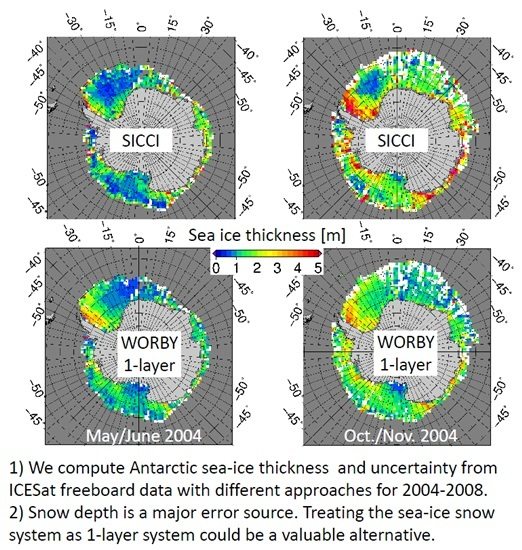
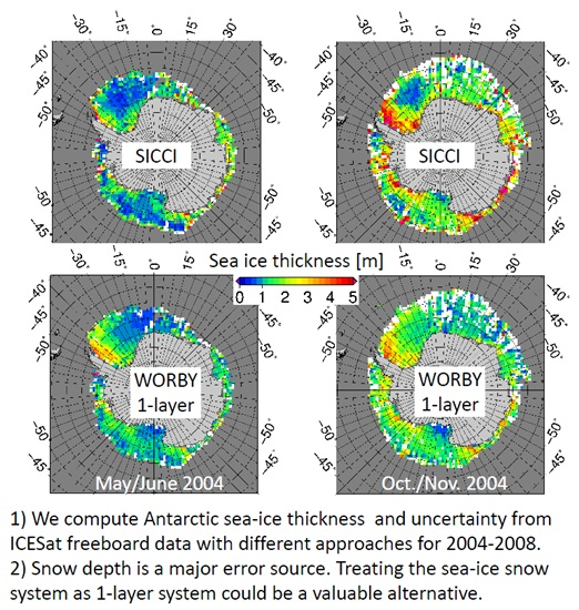
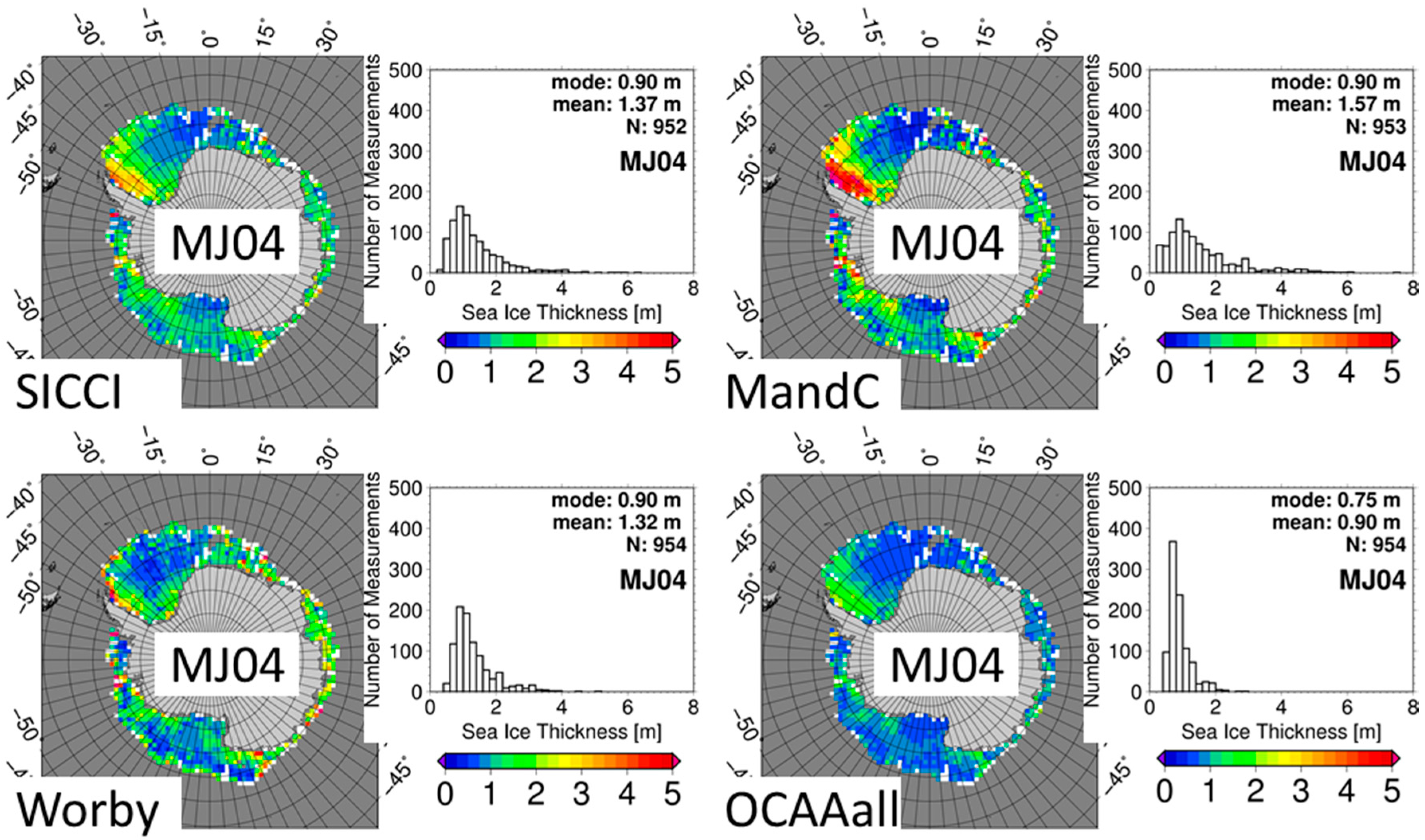
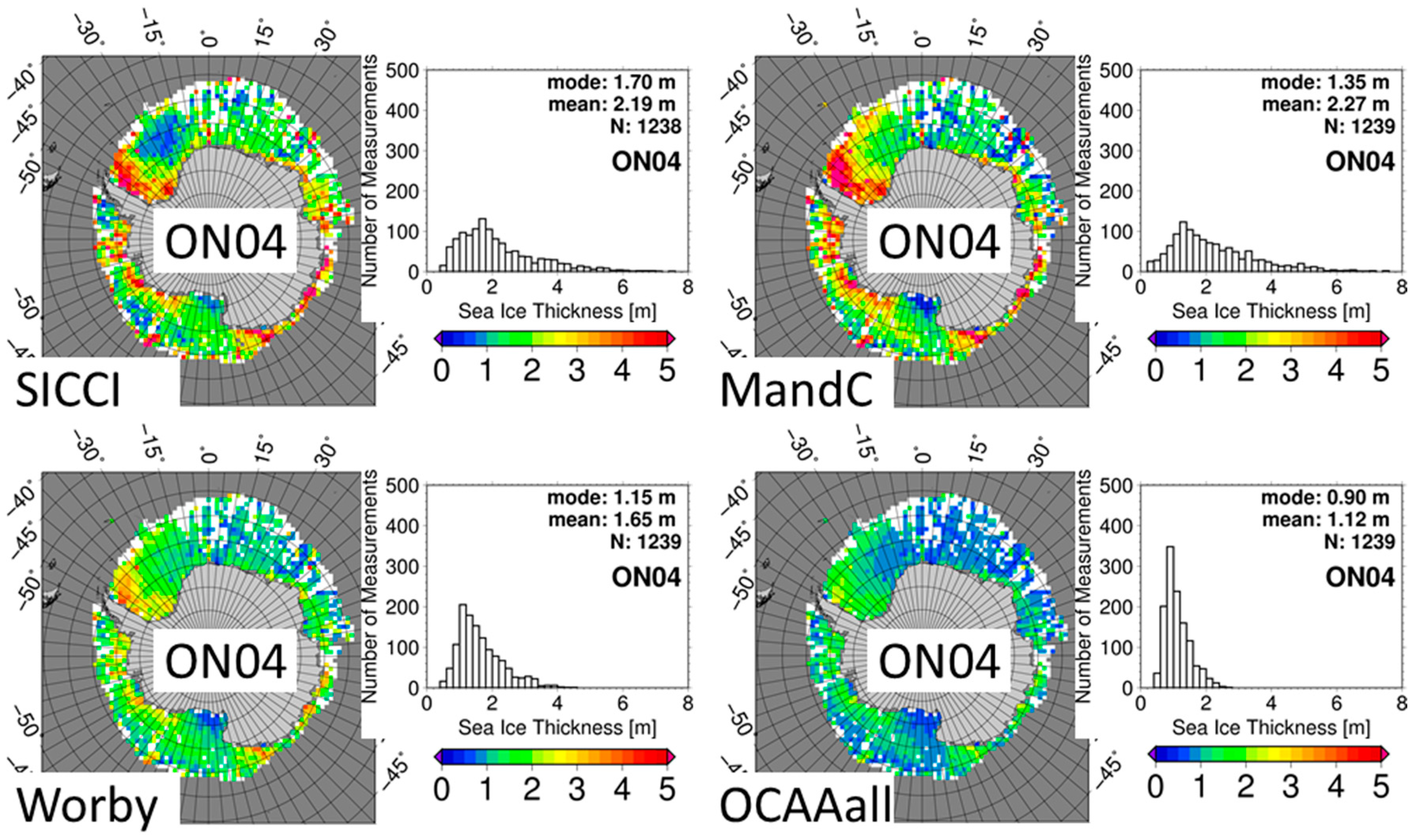
We compute Antarctic sea-ice thickness from ICESat laser altimeter observations which provide total (sea ice + snow) freeboard. We investigate four different approaches, which are based on Archimedes’ principle; only one of these (SICCI) requires actual snow depth information. The other three either use climatological snow depth information (MandC), assume that ICESat freeboard equals snow depth (KandM), or assume a one-layer system in which the impact of snow on sea ice is represented by a modified sea-ice density (Worby). In addition, we investigate empirical approaches (OC2013) which allow computation of sea-ice thickness directly from total freeboard and which neither require snow depth nor densities [4]. We compute sea-ice thickness for ICESat measurement periods between 2004 and 2008 at 100 km grid resolution. We focus on winter and spring periods. The results are inter-compared with each other and discussed qualitatively in view of the limited amount of independent sea-ice thickness information. Data sets of the sea-ice thickness retrieved with the SICCI and the Worby 1-layer approach are provided as supplementary material to this article and can also be accessed from the Integrated Climate Data Center (http://icdc.zmaw.de/1/projekte/eas-sea-ice-ecv0.html). Our main conclusions are as follows:
(i)
The main limitation of approaches like SICCI and MandC is the lack of accurate reliable snow depths. Available snow-depth data sets are based on satellite microwave radiometry. For these, snow depth is underestimated for deformed sea ice and potentially also for flooded sea ice, i.e., regions of negative sea-ice freeboard. For the snow-depth data set used in this paper, the winter-to-spring snow-depth evolution also does not seem to be correct [34]. A snow depth which is biased low explains the observed overestimation of sea-ice thickness, particularly for spring, and also the observed too large winter-to-spring increase in modal sea-ice thickness. However, the main limitation of the SICCI approach is at the same time its main advantage. Only by incorporating information about the snow depth which is contemporary to the freeboard observations one can properly resolve the smaller-scale sea-ice thickness variations.
(ii)
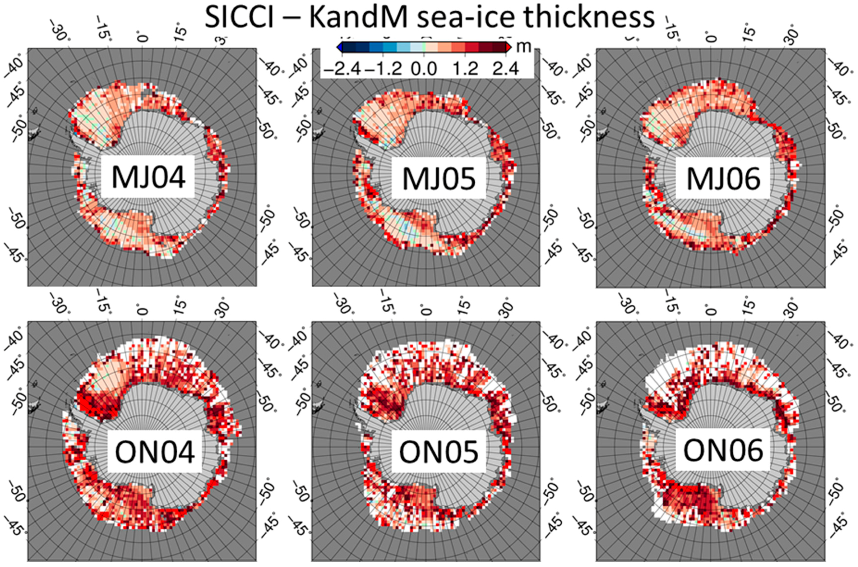
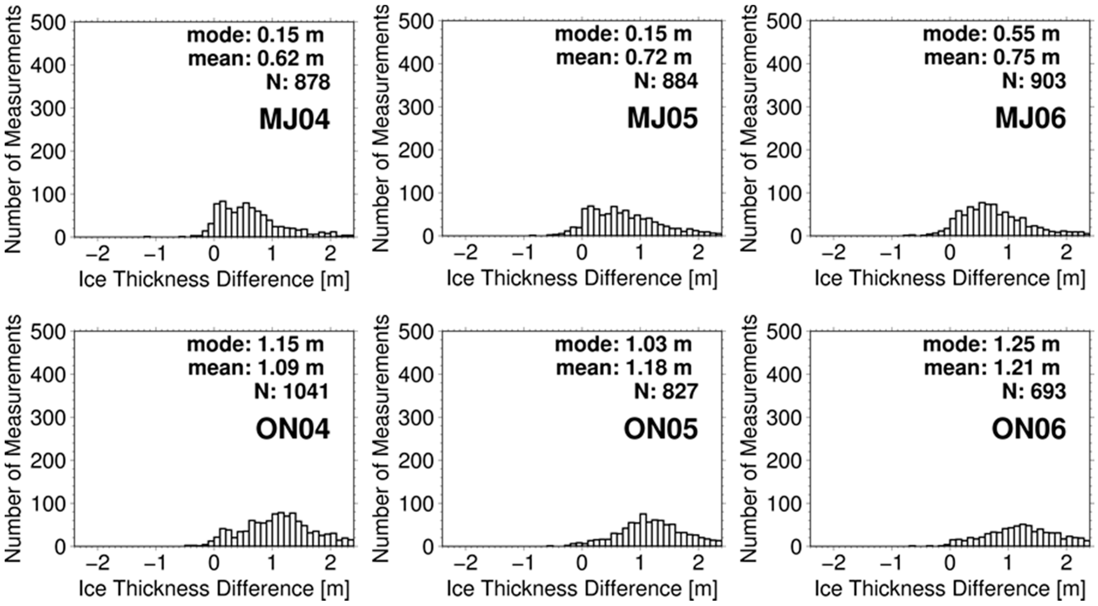
An approach like KandM, where the observed total freeboard is assumed to equal the snow depth (=sea-ice freeboard is assumed to be zero) has the potential to provide more accurate sea-ice thickness estimates than SICCI in regions where (1) the above-mentioned assumption is valid and where (2) the snow depth used by the SICCI approach is biased. We find, however, that the average KandM sea-ice thickness is too small in comparison to the other approaches (Section 3.1 and Section 3.2) and to available independent sea-ice thickness observations (Section 4.5)—in agreement to [33]. The same applies to the empirical OC2013 approaches (Section 3.2), except the one denoted OCEA which is based on measurements obtained in the East Antarctic sector (see Figure 1, right).
(iii)
Our conceptually new attempt to derive sea-ice thickness, which takes the sea ice-snow system as one layer (Worby), provides sea-ice thickness values which seem to be consistent with independent observations and with regard to the winter-to-spring sea-ice thickness evolution (Section 3.2 and Section 4.5). For this approach we assume that the density of the one-layer system with a thickness equaling snow depth plus sea-ice thickness can be described as a linear combination of the densities of snow and sea ice (see Section 2.2.5).
Currently used sea ice and snow densities need to be reviewed and potentially revised. Recent results from expeditions point to sea-ice densities which might be considerably lower and more variable than thought before [57]. Sea-ice density can cause considerable systematic uncertainties in the obtained sea-ice thickness as illustrated in Section 4.4.
The above-mentioned limitations might also apply for sea-ice thickness retrieval planned with ICESat-2 [52]. While the design of the new sensor aboard ICESat-2 will substantially improve the accuracy of freeboard retrievals and provide improved spatial-temporal coverage [52], the limitations caused by inaccurate snow depth and other input parameters like snow and ice density could counterbalance the improvements in freeboard retrieval to be achieved with ICESat-2. In this context, we recommend to (1) Improve snow depth on sea ice estimates and provide information about precision and accuracy. We refer to [59,60] for first attempts into this direction; (2) Further investigate the potential of using a one-layer system for sea-ice thickness retrieval. For this paper, we utilize climatological values of sea-ice thickness and snow depth from visual ship-based observations [6] to derive the one-layer ice density. It would be desirable to take this information from more recent observations. Continuation of programs supporting expeditions to carry out co-ordinated ground-based, underwater equipment-based, and airborne measurements of snow and ice properties is mandatory for any further development and improvement of algorithms and the validation of the obtained results.

Supplementary Materials

The following are available online at https://www.mdpi.com/2072-4292/8/7/538/s1, Supplementary S1: Data sets of the sea-ice thickness retrieved with the SICCI and the Worby 1-layer approach.

Acknowledgments

The work was carried out within the ESA Climate Change Initiative Sea Ice (SICCI) project as an activity of the Integrated Climate Data Center (ICDC) at the Center for Earth System Research and Sustainability (CEN). Stefan Kern acknowledges support given by the Center of Excellence for Climate System Analysis and Prediction (CliSAP). Burcu Ozsoy-Çiçek appreciates support given by the Istanbul Technical University (ITU) in the field of polar research, which greatly helped to conduct this study and to realize a recent Turkish research cruise into the Antarctic. This research was supported by the Antarctic Climate and Ecosystems Cooperative Research Centre (ACE CRC). The authors acknowledge support from the International Space Science Institute (ISSI), Bern, Switzerland, under project No. 245: Heil, P., and S. Kern, “Towards an integrated retrieval of Antarctic sea ice volume”. The authors thank four reviewers for their very helpful comments.

Author Contributions

Stefan Kern and Burcu Ozsoy-Çiçek analyzed the data; Stefan Kern, Burcu Ozsoy-Çiçek, and Anthony P. Worby contributed materials/analysis tools; Stefan Kern wrote the paper.

Conflicts of Interest

The authors declare no conflict of interest. The founding sponsors had no role in the design of the study; in the collection, analyses, or interpretation of data; in the writing of the manuscript, and in the decision to publish the results.

Abbreviations

The following abbreviations are used in this manuscript:
AAallentire Antarctic
AMSR-EAdvanced Microwave Scanning Radiometer aboard EOS
ARISEAntarctic Remote Ice Sensing Experiment
ARTISTArctic Radiation and Turbulence Interaction Study
ASIARTIST Sea Ice
ASPeCtAntarctic Sea ice Processes and Climate
AUVAutonomous Underwater Vehicle
EAEastern Antarctic
EMElectromagnetic induction
EOSEarth Observation Satellite
FMFebruary/March
GLASGeoscience Laser Altimeter System
GLOBECGlobal Oceans Ecosystems Dynamics
ICESatIce Cloud and land Elevation Satellite
ISPOLIce Station Polarstern
MJMay/June
NSIDCNational Snow and Ice Data Center
OIBOperation Ice Bridge
ONOctober/November
RMSDRoot Mean Squared Difference
SARSynthetic Aperture Radar
SICSea Ice Concentration
SICCIClimate Change Initiative Sea Ice project
SIMBASea Ice Mass Balance in the Antarctic
SIPEXSea Ice Physics and Ecosystem Experiment
SMOSSoil Moisture and Ocean Salinity
SSM/ISpecial Sensor Microwave/Imager
ULSUpward Looking Sonar
WWSWestern Weddell Sea

References

  1. Parkinson, C.L. Global sea ice coverage from satellite data: Annual cycle and 35-yr trends. J. Clim. 2014, 27, 9377–9382. [Google Scholar] [CrossRef]
  2. Parkinson, C.L.; Cavalieri, D.J. Antarctic sea ice variability and trends, 1979–2010. Cryosphere 2012, 6, 871–880. [Google Scholar] [CrossRef]
  3. Massonnet, F.; Mathiot, P.; Fichefet, T.; Goosse, H.; König Beatty, C.; Vancoppenolle, M.; Lavergne, T. A model reconstruction of the Antarctic sea-ice thickness and volume changes over 1980–2008 using data assimilation. Ocean Model. 2013, 64, 67–75. [Google Scholar] [CrossRef]
  4. Ozsoy-Cicek, B.; Ackley, S.F.; Xie, H.; Yi, D.; Zwally, J. Sea-ice thickness retrieval algorithms based on in-situ surface elevation and thickness values for application to altimetry. J. Geophys. Res. Oceans 2013, 118, 3807–3822. [Google Scholar] [CrossRef]
  5. Worby, A.P.; Allison, I. A Ship-Based Technique for Observing Antarctic Sea Ice: Part I Observational Techniques and Results; Research Report No. 14; Antarctic Cooperative Research Centre: Hobart, TAS, Australia, 1999; Volume 14, p. 63. [Google Scholar]
  6. Worby, A.P.; Geiger, C.A.; Paget, M.J.; Van Woert, M.L.; Ackley, S.F.; DeLiberty, T.L. The thickness distribution of Antarctic sea ice. J. Geophys. Res. 2008, 113. [Google Scholar] [CrossRef]
  7. Beitsch, A.; Kern, S.; Kaleschke, L. Comparison of SSM/I and AMSR-E sea ice concentrations with ASPeCt ship observations around Antarctica. IEEE Trans. Geosci. Remote Sens. 2015, 53, 1985–1996. [Google Scholar] [CrossRef]
  8. Harms, S.; Fahrbach, E.; Strass, V.H. Sea ice transports in the Weddell Sea. J. Geophys. Res. 2001, 106, 9057–9073. [Google Scholar] [CrossRef] [Green Version]
  9. Behrendt, A.; Dierking, W.; Fahrbach, E.; Witte, H. Sea ice draft in the Weddell Sea measured by upward looking sonars. Earth Syst. Sci. Data 2013, 5, 209–226. [Google Scholar] [CrossRef] [Green Version]
  10. Williams, G.; Maksym, T.; Wilkinson, J.; Kunz, C.; Murphy, C.; Kimball, P.; Singh, H. Thick and deformed Antarctic sea ice mapped with autonomous underwater vehicles. Nat. Geosci. 2015, 8, 61–67. [Google Scholar] [CrossRef]
  11. DeLiberty, T.L.; Geiger, C.A.; Ackley, S.F.; Worby, A.P.; Van Woert, M.L. Estimating the annual cycle of sea-ice thickness and volume in the Ross Sea. Deep Sea Res. 2011, 58, 1250–1260. [Google Scholar] [CrossRef]
  12. Bernstein, R.; Geiger, C.A.; DeLiberty, T.L.; Lemcke-Stampone, M.D. Antarctic sea-ice thickness and volume estimates from ice charts between 1995 and 1998. Ann. Glaciol. 2015, 56, 383–393. [Google Scholar] [CrossRef]
  13. Tamura, T.; Ohshima, K.I.; Enomoto, H.; Tateyama, K.; Muto, A.; Ushio, S.; Massom, R.A. Estimation of thin sea-ice thickness from NOAA AVHRR data in a polynya off the Wilkes Land coast, East Antarctica. Ann. Glaciol. 2006, 44, 269–274. [Google Scholar] [CrossRef]
  14. Tamura, T.; Ohshima, K.I.; Markus, T.; Cavalieri, D.J.; Nihashi, S.; Hirasawa, N. Estimation of thin ice thickness and detection of fast ice from SSM/I data in the Antarctic Ocean. J. Atmos. Ocean. Technol. 2007, 24, 1757–1772. [Google Scholar] [CrossRef]
  15. Martin, S.; Drucker, R.S.; Kwok, R. The areas and ice production of the western and central Ross Sea polynyas, 1992–2002, and their relation to the B-15 and C-19 iceberg events of 2000 and 2002. J. Mar. Syst. 2007, 68, 201–214. [Google Scholar] [CrossRef]
  16. Nihashi, S.; Ohshima, K.I. Circumpolar mapping of Antarctic coastal polynyas and landfast sea ice: Relationship and variability. J. Clim. 2015, 28, 3650–3670. [Google Scholar]
  17. Nakamura, K.; Wakabayashi, H.; Uto, S.; Uhsio, S.; Nishio, F. Observation of sea-ice thickness using ENVISAT data from Lützow-Holm Bay, East Antarctica. IEEE Geosci. Remote Sens. Lett. 2009, 6, 277–281. [Google Scholar] [CrossRef]
  18. Aulicino, G.; Fusco, G.; Kern, S.; Budillon, G. Estimation of sea-ice thickness in Ross and Weddell Seas from SSM/I brightness temperatures. IEEE Trans. Geosci. Remote Sens. 2014, 52, 4122–4140. [Google Scholar] [CrossRef]
  19. Tian-Kunze, X.; Kaleschke, L.; Maaß, N.; Mäkynen, M.; Serra, N.; Drusch, M.; Krumpen, T. SMOS-derived thin sea-ice thickness: Algorithm baseline, product specification and initial verification. Cryosphere 2014, 8, 997–1018. [Google Scholar] [CrossRef] [Green Version]
  20. Wadhams, P.; Parmiggiani, F.F.; de Cariolis, G.; Desiderio, D.; Doble, M.J. SAR imaging of wave dispersion in Antarctic pancake ice and its use in measuring ice thickness. Geophys. Res. Lett. 2004, 31. [Google Scholar] [CrossRef]
  21. Doble, M.J.; de Cariolis, G.; Meylan, M.H.; Bidlot, J.-R.; Wadhams, P. Relating wave attenuation to pancake ice thickness using field measurements and model results. Geophys. Res. Lett. 2015, 42, 4473–4481. [Google Scholar] [CrossRef]
  22. Laxon, S.W.; Peacock, N.; Smith, D. High interannual variability of sea-ice thickness in the Arctic region. Nature 2003, 425, 947–950. [Google Scholar] [CrossRef] [PubMed]
  23. Laxon, S.W.; Giles, K.A.; Ridout, A.L.; Wingham, D.J.; Willatt, R.; Cullen, R.; Kwok, R.; Schweiger, A.; Zhang, J.; Haas, C.; et al. CryoSat-2 estimates of Arctic sea-ice thickness and volume. Geophys. Res. Lett. 2013, 40, 732–737. [Google Scholar] [CrossRef]
  24. Giles, K.A.; Laxon, S.W.; Worby, A.P. Antarctic sea ice elevation from satellite radar altimetry. Geophys. Res. Lett. 2008, 35. [Google Scholar] [CrossRef]
  25. Willatt, R.C.; Giles, K.A.; Laxon, S.W.; Stone-Drake, L.; Worby, A.P. Field investigations of Ku-Band radar penetration into snow cover on Antarctic sea ice. IEEE Trans. Geosci. Remote Sens. 2010, 48, 365–372. [Google Scholar] [CrossRef]
  26. Schwegmann, S.; Rinne, E.; Ricker, R.; Hendricks, S.; Helm, V. About the consistency between Envisat and CryoSat-2 radar freeboard retrieval over Antarctic sea ice. Cryosphere 2015, 9, 4893–4923. [Google Scholar] [CrossRef]
  27. Markus, T.; Massom, R.A.; Worby, A.P.; Lytle, V.I.; Kurtz, N.; Maksym, T. Freeboard, snow depth and sea-ice roughness in East Antarctica from in situ and multiple satellite data. Ann. Glaciol. 2011, 52, 242–248. [Google Scholar] [CrossRef]
  28. Xie, H.; Tekeli, A.E.; Ackley, S.F.; Yi, D.; Zwally, H.J. Sea-ice thickness estimations from ICESat altimetry over the Bellingshausen and Amundsen Seas, 2003–2009. J. Geophys. Res. Oceans 2013, 118, 2438–2453. [Google Scholar] [CrossRef]
  29. Zwally, H.J.; Yi, D.; Kwok, R.; Zhao, Y. ICESat measurements of sea ice freeboard and estimates of sea-ice thickness in the Weddell Sea. J. Geophys. Res. 2008, 113. [Google Scholar] [CrossRef]
  30. Yi, D.; Zwally, H.J.; Robbins, J.W. ICESat observations of seasonal and interannual variations of sea-ice freeboard and estimated thickness in the Weddell Sea, Antarctica (2003–2009). Ann. Glaciol. 2011, 52, 43–51. [Google Scholar] [CrossRef]
  31. Kern, S.; Spreen, G. Uncertainties in Antarctic sea-ice thickness retrieval from ICESat. Ann. Glaciol. 2015, 56, 107–119. [Google Scholar] [CrossRef]
  32. Kurtz, N.T.; Markus, T. Satellite observations of Antarctic sea-ice thickness and volume. J. Geophys. Res. 2012, 117. [Google Scholar] [CrossRef]
  33. Kwok, R.; Maksym, T. Snow depth of the Weddell and Bellingshausen sea ice covers from IceBridge surveys in 2010 and 2011: An examination. J. Geophys. Res. Oceans 2014, 119, 4141–4167. [Google Scholar] [CrossRef]
  34. Kern, S.; Ozsoy-Cicek, B. Satellite remote sensing of snow depth on Antarctic sea ice: An inter-comparison of two empirical approaches. Remote Sens. 2016, 8. [Google Scholar] [CrossRef]
  35. Zwally, H.J.; Schutz, R.; Bentley, C.; Bufton, J.; Herring, T.; Minster, J.; Spinhirne, J.; Ross, T. GLAS/ICESat L2 Sea Ice Altimetry Data; Version 33; National Snow and Ice Data Center: Boulder, CO, USA, 2011. [Google Scholar]
  36. Cavalieri, D.J.; Markus, T.; Comiso, J.C. AMSR-E/Aqua Daily L3 12.5 km Brightness Temperature, Sea Ice Concentration, and Snow Depth Polar Grids; National Snow and Ice Data Centre: Boulder, CO, USA, 2003. [Google Scholar]
  37. Kaleschke, L.; Lüpkes, C.; Vihma, T.; Haarpaintner, J.; Bochert, A.; Hartmann, J.; Heygster, G. SSM/I sea ice remote sensing for mesoscale ocean-atmosphere interaction analysis. Can. J. Remote Sens. 2001, 27, 526–537. [Google Scholar] [CrossRef]
  38. Kern, S.; Kaleschke, L.; Spreen, G. Climatology of the Nordic (Irminger, Greenland, Barents, Kara and White/Pechora) Seas ice cover based on 85 GHz satellite microwave radiometry: 1992–2008. Tellus 2010, 62, 411–434. [Google Scholar] [CrossRef]
  39. Knight, C.A. Formation of slush on floating ice. Cold Reg. Sci. Technol. 1988, 15, 33–38. [Google Scholar] [CrossRef]
  40. Spreen, G.; Kern, S.; Stammer, D.; Forsberg, R.; Haarpaintner, J. Satellite-based estimates of sea-ice volume flux through Fram Strait. Ann. Glaciol. 2006, 44, 321–328. [Google Scholar] [CrossRef]
  41. Maksym, T.; Markus, T. Antarctic sea-ice thickness and snow-to-ice conversion from atmospheric reanalysis and passive microwave snow depth. J. Geophys. Res. 2008, 113. [Google Scholar] [CrossRef]
  42. Worby, A.P.; Markus, T.; Steer, A.D.; Lytle, V.I.; Massom, R.A. Evaluation of AMSR-E snow depth product over East Antarctic sea ice using in situ measurements and aerial photography. J. Geophys. Res. 2008, 113. [Google Scholar] [CrossRef]
  43. Markus, T.; Cavalieri, D.J. Snow depth distribution over sea ice in the southern ocean from satellite passive microwave data. In Antarctic Sea Ice: Physical Processes, Interactions and Variability; Jeffries, M.O., Ed.; AGU: Washington, DC, USA, 1998; pp. 19–39. [Google Scholar]
  44. Perovich, D.K.; Elder, B.C.; Claffey, K.J.; Stammerjohn, S.; Smith, R.; Ackley, S.F.; Krouse, H.R.; Gow, A.J. Winter sea-ice properties in Marguerite Bay, Antarctica. Deep Sea Res. II 2004, 51, 2023–2039. [Google Scholar] [CrossRef]
  45. Massom, R.A.; Worby, A.; Lytle, V. ARISE (Antarctic Remote Ice Sensing Experiment) in the East 2003: Validation of satellite-derived sea-ice data products. Ann. Glaciol. 2006, 44, 288–296. [Google Scholar] [CrossRef]
  46. Hellmer, H.H.; Haas, C.; Dieckmann, G.S.; Schröder, M. Sea ice feedbacks observed in Western Weddell Sea. EOS 2006, 87, 173–175. [Google Scholar] [CrossRef]
  47. Lewis, M.J.; Tison, J.L.; Weissling, B.; Delille, B.; Ackley, S.F.; Brabant, F.; Xie, H. Sea ice and snow cover characteristics during the winter-spring transition in the Bellingshausen Sea: An overview of SIMBA 2007. Deep Sea Res. II 2011, 58, 1019–1038. [Google Scholar] [CrossRef]
  48. Worby, A.P.; Steer, A.; Lieser, J.L.; Heil, P.; Yi, D.; Markus, T.; Allison, I.; Massom, R.A.; Galin, N.; Zwally, J. Regional-scale sea-ice and snow thickness distributions from in situ and satellite measurements over East Antarctica during SIPEX 2007. Deep Sea Res. II 2011, 58, 1125–1136. [Google Scholar] [CrossRef]
  49. Weissling, B.P.; Ackley, S.F. Antarctic sea-ice altimetry: Scale and resolution effects on derived ice thickness distribution. Ann. Glaciol. 2011, 52, 225–232. [Google Scholar] [CrossRef]
  50. Kwok, R.; Cunningham, G.F. Variability of Arctic sea-ice thickness and volume from CryoSat-2. Philos. Trans. R. Soc. A 2015, 373. [Google Scholar] [CrossRef] [PubMed]
  51. Connor, L.N.; Farrell, S.L.; McAdoo, D.C.; Krabill, W.B.; Manizade, S. Validating ICESat over thick sea ice in the Northern Canada Basin. IEEE Trans. Geosci. Remote Sens. 2013, 51, 2188–2200. [Google Scholar] [CrossRef]
  52. Farrell, S.L.; Brunt, K.M.; Ruth, J.M.; Kuhn, J.M.; Connor, L.N.; Walsh, K.M. Sea-ice freeboard retrieval using digital photon-counting laser altimetry. Ann. Glaciol. 2015, 56, 167–174. [Google Scholar] [CrossRef]
  53. Geiger, C.; Müller, H.-R.; Samluk, J.P.; Bernstein, E.R.; Richter-Menge, J. Impact of spatial aliasing on sea-ice thickness measurements. Ann. Glaciol. 2015, 56, 353–362. [Google Scholar]
  54. Brucker, L.; Markus, T. Arctic-scale assessment of satellite passive microwave-derived snow depth on sea ice using Operation Ice Bridge airborne data. J. Geophys. Res. Oceans 2013, 118, 2892–2905. [Google Scholar] [CrossRef]
  55. Willmes, S.; Haas, C.; Nicolaus, M.; Bareiss, J. Satellite microwave observations of the interannual variability of snowmelt on sea ice in the Southern Ocean. J. Geophys. Res. 2009, 114. [Google Scholar] [CrossRef] [Green Version]
  56. Voss, S.; Heygster, G.; Ezraty, R. Improving sea ice type discrimination by the simultaneous use of SSM/I and scatterometer data. Polar Res. 2003, 22, 35–42. [Google Scholar] [CrossRef]
  57. Hutchings, J.K.; Heil, P.; Lecomte, O.; Stevens, R.; Steer, A.; Lieser, J.L. Comparing methods of measuring sea-ice density in the East Antarctic. Ann. Glaciol. 2015, 56, 77–82. [Google Scholar] [CrossRef]
  58. Haas, C.; Jochmann, P. Continuous EM and ULS thickness profiling in support of ice force measurements. In Proceedings of the 17th International Conference on Port and Ocean Engineering under Arctic Conditions, POAC’03, Trondheim, Norway, 16–19 June 2003; pp. 849–856.
  59. Frost, T.; Heygster, G.; Kern, S. ANT D1.1 Passive Microwave Snow Depth on Antarctic Sea Ice Assessment; ESA-CCI Sea Ice ECV Project Report, SICCI-ANT-PMW-SDASS-11-14; European Space Agency: Paris, France, 2014; p. 166. [Google Scholar]
  60. Kern, S.; Frost, T.; Heygster, G. ANT D1.3 Product User Guide (PUG) for Antarctic Snow Depth Product SD v1.1; ESA-CCI Sea Ice ECV Project Report, SICCI-ANT-SD-PUG-14-08; European Space Agency: Paris, France, 2014; p. 15. [Google Scholar]
Figure 1. ICESat total freeboard derived with the SICCI approach for one winter: MJ05 (left) and one spring period: ON06 (right). White grid cells denote regions with missing ICESat data but sea-ice concentrations >60%. Grid resolution is 25 km. Solid and dashed lines paralleling meridians in the right image enclose the sectors Western Weddell Sea (WWS) and East Antarctic (EA), respectively, which are mentioned in the context of the empirical sea-ice thickness retrieval following [4].
Remotesensing 08 00538 g001
Figure 2. Circum-Antarctic sea-ice thickness distribution from SICCI (left column) and from KandM (right column) for winter (MJ04) and spring (ON04) 2004. White grid cells denote sea-ice concentration >60% but no valid ICESat freeboard retrievals. Grid cell size is 100 km. Each map is accompanied by a histogram showing the sea-ice thickness distribution using bins of 0.2 m width. In each histogram the modal and mean sea-ice thickness is given together with the number N of sea-ice thickness values falling within the value range shown.
Remotesensing 08 00538 g002
Figure 3. Circum-Antarctic ICESat sea-ice thickness difference SICCI minus KandM for winter (top) and spring (bottom) of years 2004 to 2006. White grid cells denote sea-ice concentration >60% but no valid sea-ice thickness data in either of the two sea-ice thickness data sets used. Grid cell size is 100 km.
Remotesensing 08 00538 g003
Figure 4. Histograms of the difference SICCI minus KandM sea-ice thickness for winter (top) and spring (bottom) of years 2004 to 2006 as shown in Figure 3. Binsize is 0.1 m. In each histogram the modal and mean sea-ice thickness is given together with the number N of sea-ice thickness values falling within the value range ±3.0 m.
Remotesensing 08 00538 g004
Figure 5. Circum-Antarctic sea-ice thickness distribution for—from top left clockwise—SICCI, MandC (Section 2.2.4, climatological snow depth), OCAAall (Section 2.2.3, empirical) and Worby (Section 2.2.5, one-layer) for period MJ04. White grid cells denote sea-ice concentration >60% but not enough valid sea-ice thickness data. Grid cell size is 100 km. Each map is accompanied by a histogram showing the sea-ice thickness distribution using bins of 0.2 m width. In each histogram the modal and mean sea-ice thickness is given together with the number N of sea-ice thickness values within the range shown. Note that OC2013AAall is abbreviated with OCAAall.
Remotesensing 08 00538 g005
Figure 6. Circum-Antarctic sea-ice thickness distribution for—from top left clockwise—SICCI, MandC (Section 2.2.4, climatological snow depth), OCAAall (Section 2.2.3, empirical) and Worby (Section 2.2.5, one-layer) for period ON04. White grid cells denote sea-ice concentration >60% but not enough valid sea-ice thickness data. Grid cell size is 100 km. Each map is accompanied by a histogram showing the sea-ice thickness distribution using bins of 0.2 m width. In each histogram the modal and mean sea-ice thickness is given together with the number N of sea-ice thickness values within the range shown. Note that OC2013AAall is abbreviated with OCAAall.
Remotesensing 08 00538 g006
Figure 7. Circum-Antarctic sea-ice thickness distribution for OC2013: from top to bottom: OCAAall, OCEA, and OCWWS (Section 2.2.3, empirical, see Table 2) for period MJ04 (left) and ON04 (right). White grid cells denote sea ice concentration >60% but not enough valid sea-ice thickness data. Grid cell size is 100 km. Each map is accompanied by a histogram showing the sea-ice thickness distribution using bins of 0.2 m width. In each histogram the modal and mean sea-ice thickness is given together with the number N of sea-ice thickness values falling within the range shown.
Remotesensing 08 00538 g007
Figure 8. SICCI sea-ice thickness retrieval uncertainty for MJ04 (left) and ON04 (right). White grid cells denote sea-ice concentration >60% but not enough valid sea-ice thickness data. Grid cell size is 100 km. Each map is accompanied by a histogram of the uncertainty distribution using bins of 0.1 m width. In each histogram the modal and mean uncertainty is given together with the number N of sea-ice thickness uncertainties within the range shown, i.e., 0 to 4 m.
Remotesensing 08 00538 g008
Figure 9. Histograms of circum-Antarctic total freeboard derived at 25 km grid resolution from ICESat for winter (left 2 columns) and spring (right 2 columns) for SICCI (respective left column) and KandM (respective right column). Filled and open bars in KandM histograms denote contributions from all grid cells and only the grid cells co-located with SICCI grid cells, respectively. The difference between the open and filled bars illustrates the effect of the kriging interpolation used by [32].
Remotesensing 08 00538 g009
Table 1. ICESat measurement periods used. Abbreviations given in parentheses in each cell are used throughout the paper to denote the respective period.
YearSpring (ON)Fall (FM)Winter (MJ)
20043 October–8 November (ON04)17 February–21 March (FM04)18 May–21 June (MJ04)
200521 October–24 November (ON05)17 February–24 March (FM05)20 May–23 June (MJ05)
200625 October–27 November (ON06)22 February–27 March (FM06)24 May–26 June (MJ06)
20072 October–5 November (ON07)12 March–14 April (MA07)--
2008--17 February–21 March (FM08)--
Table 2. Slope and intercept values of the three selected linear regressions for Western Weddell Sea (WWS), Eastern Antarctic (EA) (see Figure 1, right) and the entire Antarctic (AAall) together with conservative uncertainty estimates for slope and intercept of the two single regions. For region AAall the uncertainty estimate is based on the average slope and intercept uncertainties of all five regions. Intercept and intercept error are given in centimeters.
RegionSlope: aSlope Error: daIntercept: bIntercept Error: db
WWS2.340.3 × a22.010.0
EA3.500.3 × a 26.010.0
AAall2.773 × 0.4520.73 × 3.6
Table 3. Modal and mean circum-Antarctic total freeboard (in centimeters) obtained from ICESat using the SICCI approach (Section 2.2.1). Fmodal25 and Fmodal100 denote the modal values at 25 km and 100 km, respectively; Fmean25 and Fmean100 denote the corresponding mean values.
FreeboardMJ04ON04MJ05ON05MJ06ON06ON07
Fmodal2519241921182424
Fmodal10018232122182623
Fmean2526342731253332
Fmean10025332831263331
Table 4. Multi-annual seasonal average modal and mean difference SICCI minus KandM sea-ice thickness (in meter) at 100 km grid resolution. The second value in each cell is one standard deviation (in meter) of the average. N denotes the number of sea-ice thickness differences between ±3.0 m.
PeriodsFM04 to FM08MJ04 to MJ06ON04 to ON07
Modal difference0.28 ± 0.280.28 ± 0.191.15 ± 0.08
Mean difference0.77 ± 0.050.70 ± 0.061.16 ± 0.04
N162 ± 44888 ± 11910 ± 158
Table 5. Multi-annual average modal (normal font) and mean (bold font) sea-ice thickness (in meter) for winter (MJ) and spring (ON) for all approaches. The second value in each cell is one standard deviation (in meter) of the average over the 3 and 4 periods, respectively.
MethodSICCIKandMMandCWorbyOCAAallOCEAOCWWS
MJ, mode0.90 ± 0.000.43 ± 0.090.97 ± 0.090.97 ± 0.0920.73 ± 0.020.90 ± 0.000.72 ± 0.02
MJ, mean1.53 ± 0.120.66 ± 0.041.68 ± 0.111.37 ± 0.060.93 ± 0.031.18 ± 0.040.82 ± 0.03
ON, mode1.58 ± 0.160.43 ± 0.081.28 ± 0.101.14 ± 0.020.90 ± 0.001.10 ± 0.000.83 ± 0.08
ON, mean2.16 ± 0.090.70 ± 0.052.18 ± 0.081.60 ± 0.041.09 ± 0.031.38 ± 0.030.97 ± 0.02
Table 6. Multi-annual average modal and mean values of the sea-ice thickness retrieval uncertainty (in meter) for winter (MJ) and spring (ON) for SICCI and OC2013AAall computed at 100 km grid resolution. The second value in each cell is the standard deviation (in meter) of the average value.
MethodMJmodalMJmeanONmodalONmean
SICCI0.36 ± 0.010.5 ± 0.020.45 ± 0.000.55 ± 0.02
OCAAall0.25 ± 0.000.37 ± 0.010.35 ± 0.000.45 ± 0.01
Table 7. Multi-annual average modal and mean sea-ice thickness (in meter) retrieved with SICCI for three different sea-ice density values for winter (MJ) and spring (ON). The second value in each cell is the standard deviation (in meter) of the average value.
Density (kg/m3)MJmodalMJmeanONmodalONmean
915.10.90 ± 0.001.53 ± 0.121.58 ± 0.162.16 ± 0.09
900.00.72 ± 0.161.35 ± 0.101.44 ± 0.111.90 ± 0.08
875.00.63 ± 0.131.12 ± 0.091.18 ± 0.081.58 ± 0.07
Table 8. Values of R used to compute the one-layer ice density ρ ice * for all Antarctic regions used in [6] and the entire Southern Ocean for fall (FM), winter (MJ), and spring (ON). ρ ice * is derived based on a sea-ice density of 915.1 kg/m3.
PeriodFMMJON
Region (after [6])R ρ ice * (kg/m3)R ρ ice * (kg/m3)R ρ ice * (kg/m3)
Ross Sea6.38314.88093.7784
Western Weddell Sea7.3841----5.5820
Eastern Weddell Sea8.88526.88365.6822
Indian Ocean Sector6.48324.98116.0827
Pacific Ocean Sector6.88366.08275.2816
Bellingshausen/Amundsen Sea----5.98264.6805
Entire Southern Ocean6.88366.08275.4819
Table 9. Multi-annual average modal and mean sea-ice thickness (in meter) retrieved with Worby using the minimum, the maximum, and the entire Antarctic R value for winter (MJ) and spring (ON). The second value in each cell is the standard deviation (in meter) of the average value.
PeriodMJmodalMJmeanONmodalONmean
Entire Antarctic0.97 ± 0.091.37 ± 0.061.14 ± 0.021.60 ± 0.04
Minimum0.90 ± 0.001.25 ± 0.061.05 ± 0.091.37 ± 0.04
Maximum1.05 ± 0.111.43 ± 0.061.26 ± 0.061.67 ± 0.04

