Presentation Transcript

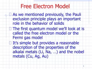
1. Quantum Free Electron Model • Sommerfeld, in 1928, applied the principle of quantum Mechanics to the Drude’s proposal of free electron gas. • According to Sommerfeld’s model a valance electron moves freely in a constant potential within the boundaries of the metal and it is prevented from escaping the metal by very high potential at the boundaries. In other words electrons are trapped in a potential well. He assumed that a moving electron behaves as if it is a system of waves, called matter waves. • By this theory Sommerfeld correctly predicted the values of specific heat of metals, electrical conductivity and thermal conductivity of metals. • Only Fermi electrons are responsible for electrical conductivity and other properties.

2. The problem is solved by quantum mechanically to find the possible values of energy possessed by the electron. • To find the how the electrons are distributed among the different possible energy levels, For this purpose Sommerfeld employed Fermi – Dirac Statics instead of Maxwell – Bolzmann statics. • Taking zero for the constsnt value of the potential inside the metal specimen, we solve the time independent wave equation to get the possible energy values En of the electrons. This is similar as that of a particle in a potential box. • In case of three dimensional n2 = nx2 + ny2 + nz2. • Thus solution of the Schodinger equation tell us what are the energy states available for the electron.

3. The three integers nx, ny, nz are called quantum numbers, which specify completely each energy state. Since for a electron inside the metal, c cannot be zero, no quantum number can be zero. The energy depends on the sum of the squares of the quantum numbers nx, ny, nz and not on their individual value. Several combinations of the three quantum numbers may give numbers may give different wave functions, but of the same energy value. Such sates and energy levels are said to be degenerate.

5. The Energy Distribution Function The distribution function f(E) is the probability that a particle is in energy state E. The distribution function is a generalization of the ideas of discrete probability to the case where energy can be treated as a continuous variable. Three distinctly different distribution functions are found in nature. The term A in the denominator of each distribution is a normalization term which may change with temperature. • Maxwell Bolzmann distribution function: Identical but distinguishable particles: Example:- gas molecules • Bose – Einstein distribution: Indistinguishable and nonexclusive particles: Example:- Photons, a particles • Fermi-Dirac distribution:- Indistinguishable and mutually exclusive particles.

6. Fermions Fermions are particles which have half-integer spin and therefore are constrained by the Pauli exclusion principle. Particles with integer spin are called bosons. Fermions include electrons, protons, neutrons.

7. The Fermi-Dirac Distribution At 0 deg K, the electrons are distributed in the lowest possible energy levels satisfying Pauli's Exclusion Principle.  As the temperature increases, the electrons gain energy such that some of them are able to transfer to higher energy levels.  The change in the occupancy of the energy levels as temperature increases is quantified by the Fermi-Dirac Distribution Function, which gives the probability that an energy level is occupied by an electron at absolute temperature T.  where ƒ(E) is the probability that energy level E is occupied by an electron, Ef is the Fermi Energy, and k is Boltzmann's constant

9. At absolute zero K, there is zero probability that an electron will occupy any energy level above EF. Similarly, the probability that a permissible energy level below EF will be occupied by an electron is 1.

10. As temperature increases above absolute zero, the distribution of electrons in a material changes.  At T > 0 deg K, there is a non-zero probability that permissible energy levels above EF would be occupied, in the same way that there is non-zero probability that energy levels below EF would be empty. In fact, the probability that an energy level above EF is occupied increases with temperature. The diagram shows the probability of an energy level being occupied, or ƒ(E) vs. energy, as a function of temperature.  The figure shows that at T > 0 deg K, the plot of ƒ(E) against energy level is sigmoidal in shape.  At E = EF, the probability that the energy level is occupied by an electron is 1/2.