Initialization: Where do you start?

In part 1 of this series, we introduced K-means clustering. We ended with an overview of the algorithm which involved repeatedly updating cluster labels and cluster centroids until they settled down to a stable configuration, but we postponed the discussion of one crucial step: where to start. That is the focus of this post.

There are a variety of initialization methods for \(K\)-means clustering. The existence of different initialization techniques points to one weakness of K-means clustering: the final clustering is very much dependent on how you start. This dependence reveals itself in two ways:

• Different initializations can lead to different final clusterings of different quality. That is, one set of clusters may be more tightly packed than the other. In more technical terms, the within cluster variation of the resulting clusters are different.
• Even when two initializations result in the same final clustering, one may require many more steps to get there.

The goal of this post is to look at a few different initialization techniques and some things that can go wrong in the the K-means algorithm. Our goal is exploration, so you should be careful not to generalize too much from the examples. In particular, we'll be working with toy data sets in 2-dimensions and will not have to worry about the curse of dimensionality.

For a more thorough survey of different initialization methods, see the paper A Comparative Study of Efficient Initialization Methods for the K-Means Clustering Algorithm by Celebi, Kingravi, and Vela.

The Jupyter notebook containing the code for part 1 of this series has been expanded to include the code for the second part as well.

Random Methods

We will look at the following three initialization methods:

• Random partition: Initialize the labels by randomly assigning each data point to a cluster.
• Random points: Initialize the centroids by selecting \(K\) data points uniformly at random.
• \(K\)-means++: Initialize the centroids by selecting \(K\) data points sequentially following a probability distribution determined by the centroids that have already been selected.

A note about the terminology: Different authors have referred to both the random partition method and the random points method as Forgy initialization after Edward Forgy. Celebi et al maintain that Forgy introduced the random partition method and that the random points method was introduced by James MacQueen. We'll try to avoid mis-attribution and confusion by using the names above.

The Scikit-Learn KMeans function allows for three different initialization techniques including K-means++ (the default) and random points (simply called random). For the third initialization method, you can directly provide an array of initial cluster labels.

A key feature of these three methods is that the initialization involves some randomness. As mentioned above and as we'll see below in more detail, it is possible for different initializations to converge to different solutions. One way to deal with this problem is to run K-means several times with different random initializations (though not necessarily different initialization techniques).

The first step is random, it's true
Once it's taken, you just follow through
And times when your cluster
Results are lackluster
You're better off starting anew

Random Partition Initialization

For the random partition initialization method, we assign each point to a cluster uniformly at random.

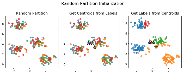
The initial centroids generated this way tend to be close together: the centroid of each cluster is an unbiased estimator of the centroid of the full data. This can be a problem if no actual data points are near the centroid of the full data. For example, the initialization below caused the number of clusters to drop.

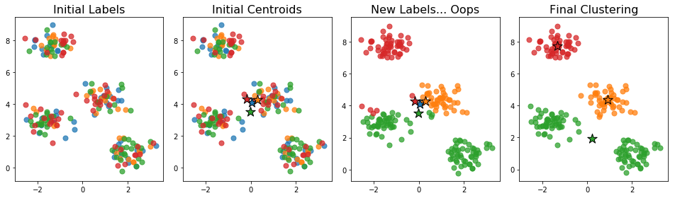
No point is closest to the initial blue centroid. This means, that when we assign labels in the next step, no point gets assigned to that cluster. The algorithm proceeds and we end up with just 3 clusters instead of the desired 4.

Consider an extreme example of this problem in 1-dimension. Suppose we have 10 evenly-sized tightly packed clusters of points concentrated at each of the odd integers from -9 to 9. If the data set is large, then when we randomly assign labels to each point, the resulting centroids are likely to be near 0. If the clusters are sufficiently tightly packed, then there will be a large interval between -1 and 1 containing no data points. In this situation, many of the clusters will disappear.

We can try and avoid the problem of empty clusters at initialization by starting with centroids that are themselves data points. This is the idea of random points initialization and it means the clusters obtained from the initial centroids will not be empty. Unfortunately, for certain data configurations, it can still happen that a cluster becomes empty at a later point in the algorithm (an example can be found here), so any implementation of K-means should address this problem in some way.

The random partition initialization method also has problems in the edge case when the number of clusters is large relative to the number of data points. For example, if we try to separate 1000 data points into 200 clusters, the random partition method will only yield the full 200 initial clusters just over 25 percent of the time. We can simulate this scenario in Python with the following block of code:

import numpy as np

# Set number of data points and clusters
datapoints = 1000
clusters = 200

# Perform a large number of trials
trials = 100000
success = 0
for i in range(trials):
    # Randomly assign labels
    assignments = np.random.choice(range(clusters), size = datapoints)
    # Check whether all labels are present
    if len(np.unique(assignments)) == clusters:
        success += 1

# Print the frequency of successful trials
print(success/trials)

Alternatively, as a fun little exercise you can calculate the exact probability using the inclusion-exclusion principle.

Random Points Initialization

In random points initialization we initialize the centroids rather than the labels. This is done by choosing K data points uniformly at random to be the initial centroids.

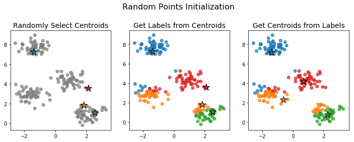
Because we're choosing the points uniformly at random, the initial centroids need not be very representative of the full data. In such cases, the algorithm can take a long time to converge or may converge to a poor clustering configuration. Below is an example an initialization that leads to a poor final clustering.

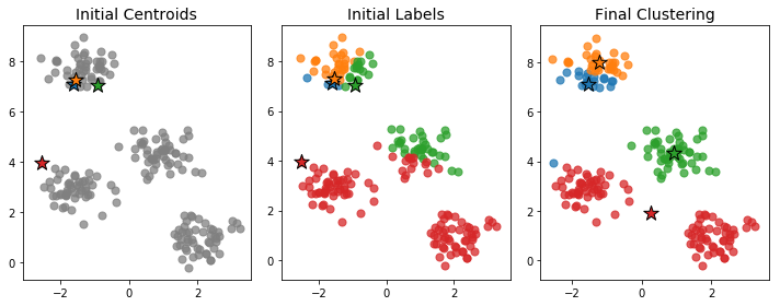
Indeed, of the four clusters, only one seems to have been correctly isolated. The two clusters near the bottom have been combined into one large red cluster, while the cluster at the top has been split into two separate blue and orange clusters.

One feature contributing to the poor clustering is the fact that the initial centroids were so close together. Having the initial centroids near each other doesn't necessarily mean we'll end up with a bad clustering, but it makes it more likely and often increases the number of steps that must be performed before the clusters settle down.

K-means++

The K-means++ initialization technique tries to avoid initial centroids that are close together.

K-means++ is similar to random points initialization, in that it selects data points at random to act as the initial centroids. However, instead of choosing these points uniformly at random, K-means++ chooses them successively in such a way as to encourage the initial centroids to be spread out. Specifically, the probability that a point will be chosen as an initial centroid is proportional to the square of its distance to the existing initial centroids.

Let's illustrate how this works with an example. To visualize the process more clearly, we'll work with a smaller dataset, consisting of only 20 data points separated into 4 clusters.

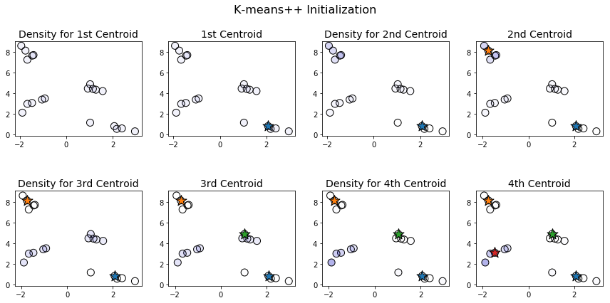
When choosing the first centroid, all points are equally likely to be chosen. This is illustrated above by the fact that all the points in the first plot have the same hue. Once the first centroid is chosen, points farthest from this centroid are most likely to be chosen for the second centroid. Notice that in the third plot on the first row, the points in the upper left corner are darker and those in the bottom right are lighter. And, indeed, the point chosen as the second centroid is one of the ones in the top left. Once we have two centroids, the points in the center and center-left become darker, while those in the top-left become lighter.

Notice that each of the initial centroids we chose is part of a different cluster. The probability of this occurring if the points are chosen uniformly at random is a little less than 13 percent (there are \(20\) choose \(4\) = \(4845\) ways of choosing 4 points and \(5^4 = 625\) ways of choosing one point from each cluster). Indeed, applying random points initialization on the same data with different random seeds gives the following initializations:

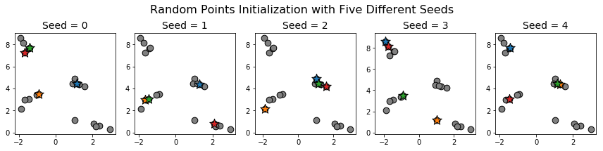
In none of these cases do we have exactly one initial centroid per cluster.

Let's compare with \(K\)-means++:

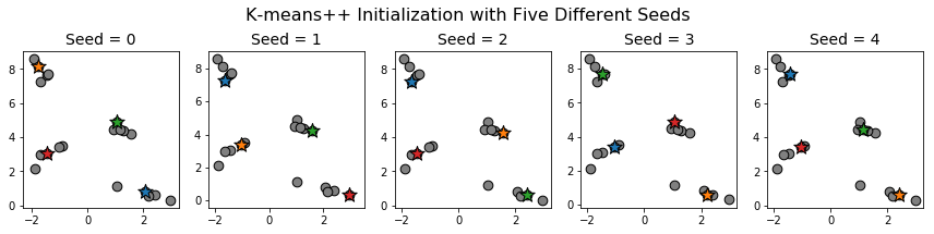
Even though the initial centroids varied from one initialization to the next, we still ended up with one centroid per cluster.

Having well separated initial centroids often causes the K-means clustering algorithm to converge more quickly. Of course, the K-means++ initialization procedure is more complicated, so there's a trade-off.

Comparing the Three Methods on our Toy Data

For each of the three methods, I ran 100 different random initializations and then carried out K-means clustering until the clusters stabilized. The results are plotted below (with a little jitter to show the frequency of different outcomes).

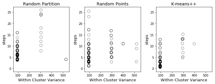
Along the x-axis, we have the within-cluster variance, which is measure of the quality of the final clusters: tightly packed clusters have lower variance, spread-out clusters have higher variance. Along the y-axis, we have the number of steps following initialization before the clusters stabilize (where a step consists of either recomputing the centroids given the labels or recomputing the labels given the centroids). Points in the lower left of the graph correspond to good initializations (quickly converge to tight clusters) while those in the upper right correspond to poor initializations (slowly converge to spread-out clusters).

The number of steps is a useful metric for gauging how well the algorithm performs once the initialization is complete, but does not reflect the complexity of the initialization. The points corresponding to K-means++ hug the lower left corner more closely than the other two initializations, but initializing K-means++ is also more complex. That being said, my experience working with data was that K-means++ was a little more efficient than the other two algorithms, taking roughly 60% as long to run completely (initialization all the way to stable clustering) as random points initialization (the slowest of the three).

Finally, I want to emphasize that the within cluster variance varied between runs for all three initialization methods. Each method obtained the minimum possible within cluster variance and each method also yielded non-optimal final clusterings. Therefore, whatever initialization technique you use, it is important to run multiple random initializations. (In Scikit-Learn, the default setting is to run 10 random initializations and return the best output of the 10.)

What's Next?

In the next part of this series, we'll look more closely at how K-means minimizes the within cluster variance and look at data sets where minimizing this variance does not capture the underlying structure in the data. Some numeric data sets are just not well suited to K-means clustering. But sometimes data can be transformed to be more amenable to K-means through tricks like standardization. In part 3, we'll discuss these topics in more detail and illustrate them with example data sets.