One of the most important lessons of QFT in curved space is that the notion of a particle is an observer-dependent concept. That’s not to say it isn’t locally useful, but without specifying the details of the mode decomposition and the trajectory/background of the detector/observer, it’s simply not meaningful. In addition to challenging our intuition, this fact lies at the heart of some of the most vexing paradoxes in physics, firewalls chief among them. In this post, I want to elucidate this issue by introducing a very important tool: the Bogolyubov (also transliterated as “Bogoliubov”) transformation.

In a nutshell, a Bogolyubov transformation relates mode decompositions of the field in different states. Consider quantizing the free scalar field in -dimensional Minkowski (i.e., flat) spacetime. From part 1, we have

where , , and the creation/annihilation operators satisfy the standard equal-time commutation relation, which in our convention is , with the vacuum state such that . (The derivation of this commutation relation, as well as the reason for splitting the normalization in this particular way when identifying the modes , will be discussed below). Typically, we choose the positive solution to the Klein-Gordon equation, , so that the operator has an interpretation as the creation operator for a positive-frequency mode traveling forwards in time. Note however that this statement depends on the existence of a global timelike Killing vector. That is, the modes are of positive frequency with respect to some time parameter , by which we mean they’re eigenfunctions of the operator with eigenvalue :

In general spacetimes however, there will be no Killing vectors with respect to which we can define positive-frequency modes, so this decomposition depends on the observer’s frame of reference. Another way to say this is that the vacuum state is not invariant under general diffeomorphisms, because these have the potential to mix positive- and negative-frequency modes. Indeed, the spirit of general relativity is that there are no privileged coordinate systems. Hence we could equally-well quantize the field with a different set of modes:

which represent excitations with respect to some other vacuum state , i.e., . Since both sets of modes are complete, they must be linear combinations of one another, i.e.,

These are the advertised Bogolyubov transformations, and the matrices , are called Bogolyubov coefficients. (Note that unlike [1], we’re working directly in the continuum, so the coefficients should be interpreted as continuous functions rather than discrete matrices). These can be determined by appealing to the normalization condition imposed by the Klein-Gordon inner product,

where the integral is performed over any Cauchy slice; for the present case of 1d flat space, . The idea behind this choice of inner product is that it allows the easy extraction of the Fourier coefficients from (1) as follows:

and similarly for ; commuting the two yields the standard commutation relation for the creation/annihilation operators above. The modes are orthonormal with respect to this inner product, and therefore provide a convenient basis for the solution space:

and similarly for , hence the funny split in the normalization we mentioned below (1) (for our notation/normalization conventions, see part 1). For example,

Taking the inner product of different sets of modes then allows one to isolate the Bogolyubov coefficients:

Explicitly:

where the second equality in the last line follows from (8); similarly for . Equating the two mode expansions (1) and (3) for the same field then leads to the following relationship between the creation/annihilation operators:

For example, the first of these is obtained by expressing everything in terms of :

Taking the Klein-Gordon product with (recall this is how we isolate the coefficients, cf. (6)), and using the fact that the modes are orthonormal (7), we then have

Note that had we taken the Klein-Gordon product with , we’d simply have obtained . To solve for the second relation, , we repeat this process, instead rewriting the left-hand side of (12) in terms of . Importantly, one can see immediately from (11) that these two quantizations, (1) and (3), lead to different Fock spaces (i.e., different vacuum states) unless . Said differently, implies that the alternative quantization is a linear combination of both positive- and negative-frequency modes with respect to the Killing vector . In this case, does not imply , so the latter quantization will detect particles when the former does not! In some sense, this is just the same spirit of relativity (i.e., no privileged reference frames) carried over to QFT, but it’s a radical conclusion nonetheless.

To make things more concrete, let’s apply this machinery to Rindler space, which describes a uniformly accelerating observer in the Minkowski background. The metric is obtained via a hyperbolic transformation of the flat space coordinates to :

which yields

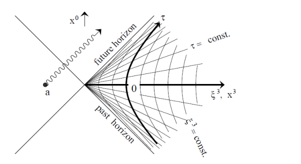
where is some constant that parametrizes the acceleration. Note however that these coordinates cover only a single quadrant of Minkowski space, namely the wedge . The line is the Rindler horizon, the physics of which well-approximates the near-horizon geometry of a black hole (when the curvature and radial directions can be ignored). This last fact underlies the central importance of Rindler space in the study of black holes, and QFT in curved space in general, as it captures many of the key features of horizons (e.g., their thermodynamic properties). Rindler time-slices — that is, lines of constant — are straight, , while lines of constant — which represent a fixed position from the horizon in these coordinates — are hyperbolae, . The proper acceleration is given by , so that the closer one gets to the horizon, the harder one has to accelerate (note again the analogy with black holes here). These hyperbolae asymptote to the null rays , so that the accelerated observer approaches the speed of light in the limit ; see the image below (I found this online, so don’t let the different labels confuse you):

 

Now, suppose we want to determine the particle spectrum that a Rindler observer would detect in the Minkowski vacuum. That is, if you were a constantly accelerating observer in empty flat space, would you still see vacuum? To answer this question, let’s compute the expectation value of the number operator for the Rindler modes in the Minkowski vacuum state, . This requires expressing the Rindler creation/annihilation operators in terms of their Minkowski counterparts, in order to figure out how they act on this state.

There’s a trick in Birrell and Davies [1], credited to Unruh, for deducing the linear combination of Minkowski modes that corresponds to a given Rindler mode that bypasses the need to work out the Bogolyubov coefficients explicitly (though the normalization must be inserted by hand, and the switch to a second, alternative set of Minkowski modes appears rather out of the blue). The basic idea is to write down the combination of Minkowski modes with the same positive-frequency analyticity properties as the Rindler modes in the desired wedged. While this is sufficient if one is only interested in knowing how the Rindler modes act on the Minkowski vacuum, working out the Bogolyubov coefficients explicitly is required in many other scenarios, and is a character-building exercise besides. Since I had to do this in the course of a previous project anyway (we wanted to compute the overlap between two states, which required commuting Rindler and Minkowski modes), I may as well share the calculation here. For simplicity, in what follows I’m going to restrict to the case of a massless scalar field. Performing the computation in and coordinates is rather tedious, and requires a case-by-case analysis depending on the signs of various momenta. A more elegant method, presented in [2] (beware, wrong sign convention!), is to first rotate to lightcone coordinates

where we’ve chosen the signs so that in the wedge under consideration. Since we’re working with massless fields, these coordinates have the significant advantage of not mixing positive and negative frequencies. That is, observe that in these coordinates, the Minkowski and Rindler metrics become, respectively,

which makes the transformation between them much simpler:

The key point is the following: since the wave equation is conformally invariant, and Rindler is conformal to Minkowski, we can write the mode expansion in terms of plane waves just as we did in the flat space case above, cf. (1). The additional simplification afforded by the use of lightcone coordinates is that the contribution from positive-frequency modes in this expansion can be directly matched to the corresponding positive-frequency contribution in flat space (similarly for the negative frequencies). The lack of mode mixing in these coordinates greatly shortens the computation of the Bogolyubov coefficients, because — in addition to avoiding the case-by-case treatment — it enables us to isolate the desired modes via a simple Fourier transform, rather than needing to perform the full Klein-Gordon inner product as above.

So, let’s split the Minkowski mode decomposition into positive- and negative-frequency parts; from (1), we have

where in the second line, we used the on-shell condition , and then in the last line changed integration variables in the second term in order to combine the integrals. In lightcone coordinates (16), this becomes

where we’ve absorbed the pesky factor of via the rescaling . Observe how the final expression naturally decomposes into creation/annihilation operators for left- and right-movers. And since the Rindler metric is conformally flat, it admits a formally identical expression within the wedge :

where is the rescaled Rindler momentum, and 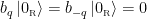. Now comes the chief advantage of this approach mentioned above: since the notion of positive/negative momenta is preserved under the conformal transformation from Minkowski to Rindler space, we can directly identify

Now, what we’re after is an expression for the Rindler operators in terms of the Minkowski operators , so that we can compute the expectation value of the number operator, . To that end, we first isolate the right-moving annihilation mode by an appropriate Fourier transform of the first of these equations:

where, a priori, we allowed the momentum in the Fourier transform to take any sign. Recalling however that the expressions (22) were derived for positive momenta, we must have

where we have defined

where in the second equality we have substituted the definition (18). We can then obtain by simply taking the hermitian conjugate of this expression, noting that by definition,

Similarly, by Fourier transforming the second equation in (22), we obtain

the hermitian conjugate of which gives .

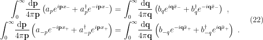
With the expressions (24), (27) for the Rindler creation/annihilation operators in terms of their Minkowski counterparts in hand, we can compute the expectation value of the Rindler number operator in the Minkowski vacuum, to determine what a uniformly accelerating observer would observe. For compactness, we shall denote in the following computation:

Now, the seemingly straightforward way to evaluate the integral over is to explicitly work out , but the latter requires a contour integral, and one is left with an integral over a product of complex Gamma functions for the former (I’ve included this at the end of this post, for the masochistic among you). A more clever alternative, taking a tip from [2], is to use the normalization condition on the Bogolyubov coefficients one obtains from the canonical commutation relations:

where in the last step we used the fact that (exercise for the reader, or see the appendix below). Since the left-hand side is equal to , we must have

and therefore, setting , we obtain

which is exactly the integral we needed in (28)! Therefore,

where in the last step, we have undone our rescaling below (20): (that is, here plays the role of the original Rindler momentum in (3). Note that the integration measure doesn’t pick up a factor of , because we really should have integrated with respect to from the very start of (28)).

This is the final answer, except for two divergences: an IR divergence , and a UV divergence due to the fact that we integrated over arbitrarily high momenta. The first is rather silly, and arises from the infinite spatial volume :

Meanwhile, the UV divergence is to be expected, since there are an infinite number of modes. We could impose a momentum cutoff on the integral to regulate this, but what we’re really after is the number density , where . Hence, stripping off the divergences in this manner, we arrive at

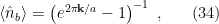
which is precisely the Plank spectrum for a black body at temperature .

This result — that a uniformly accelerating observer in Minkowski vacuum observes a thermal spectrum — is called the Unruh effect, and is nothing short of remarkable. From an operationalist standpoint, one can say that the acceleration of the Rindler observer is what provides the energy for these excitations, but this sidesteps the question of their ontological status (indeed, the closely related question of exactly how pairwise entangled Hawking modes evolve to particles in the inertial frame at infinity is a non-trivial problem to which I hope to return). In the context of the maximum entropy procedure we’ve discussed before, the thermal spectrum may be regarded as a consequence of the fact that the Rindler observer has traced-out everything on the other side of the horizon, so the only information she has left is the temperature set by her own acceleration. If we restore units, this temperature reads

The Unruh effect thus represents a deep interplay between statistical thermodynamics née information theory (), relativity (), and quantum field theory (). It is another manifestation of the thermal nature of horizons we mentioned in part 1, and arises as an inevitable consistency condition between inertial and Rindler frames. Furthermore, since the Rindler frame well-approximates the near-horizon geometry of a static black hole, the Unruh effect is intimately related to Hawking radiation, and my personal suspicion is that when we understand things more deeply, we’ll find the same underlying explanation for both. Indeed, in the Bekenstein-Hawking formula for black hole entropy , the only additional ingredient in this exceptional confluence is the presence of gravity ()—the nature of which we’re far from having grasped.

References

---

As an exercise in contour integration, one can obtain an explicit expression for the integral (25). The trick is to massage it into a gamma function:

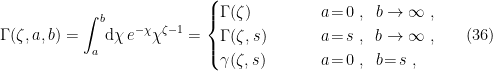
where and are the upper and lower incomplete gamma functions, respectively, and with . We then begin by defining a new variable , so that

where we have defined the rescaled momentum vectors , (and broken the boldface convention, because I didn’t want to introduce even more letters). This is pretty close to the desired form already, but the complex exponent necessitates that we promote to a complex variable, and treat this as a contour integral in the complex plane.

Recall that we can write any in the form with , which has branch points at both and , since there’s a non-trivial monodromy along a closed path that encircles either point in the complex plane. Since the integral converges as due to the exponential damping, let’s choose the branch cut to run from to along the negative real axis, so that the following contour encloses no poles:

where the arc term is a quarter-circle that connects the positive real and complex axes at , which vanishes since . Thus, taking along the positive complex axis, the integral (37) becomes

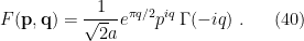
where . Comparing with the form of the gamma function (36), we identify and , whence we find

As an aside, while the form of this expression makes it non-obvious, the property (26) is preserved, as one can easily show by noting that

Substituting this result back into (24), we at last obtain

where the Bogolyubov coefficients are

The left-movers are similarly obtained from (27).

References

- N. D. Birrell and P. C. W. Davies, Quantum Fields in Curved Space. Cambridge Monographs on Mathematical Physics. Cambridge Univ. Press, Cambridge, UK, 1984. http://www.cambridge. org/mw/academic/subjects/physics/theoretical-physics-and-mathematical-physics/ quantum-fields-curved-space?format=PB.
- V. F. Mukhanov and S. Winitzki, Introduction to Quantum Fields in Classical Backgrounds. 2004. https://uwaterloo.ca/physics-of-information-lab/sites/ca. physics-of-information-lab/files/uploads/files/text.pdf. (freely-available draft of the published textbook).