LBIST is a form of built in self-test (BIST) in which the logic inside a chip can be tested on-chip itself without any expensive Automatic Test Equipment (ATE). A BIST engine is built inside the chip and requires only an access mechanism like the Test Access Port (TAP) to start.
This article will describe about the BIST architecture in brief and Test Pattern Generator (TPG) used in LBIST. And we will discuss about the output Response Analyzer (RA) in this article.
The general architecture of an on-chip BIST consists of 3 major components –
1. BIST controller
2. TPG (Test Pattern Generator)
3. RA (Response Analyzer)
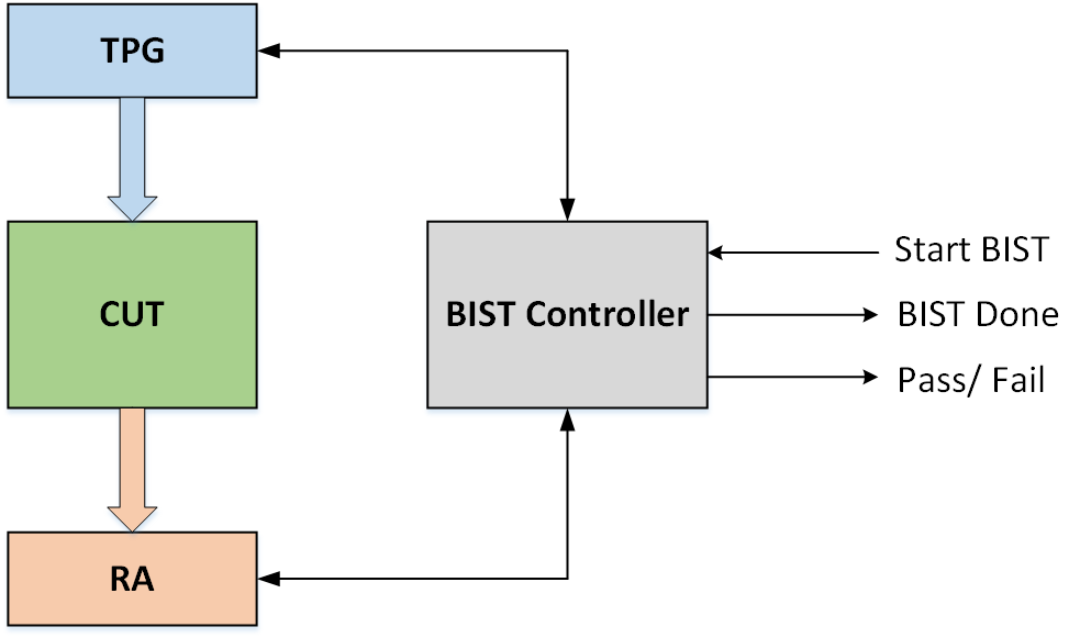
The basic mechanism of LBIST is it uses a Linear Feedback Shift Register (LFSR) to generate the inputs to the device’s internal scan chain, initiate a functional cycle to capture the response of the device, and then compress the captured response using a multiple input signature register (MISR). The compressed response that comes out of the MISR is called the signature. Any corruption in the output signature indicates a defect in the device.
Test Pattern Generator (TPG)
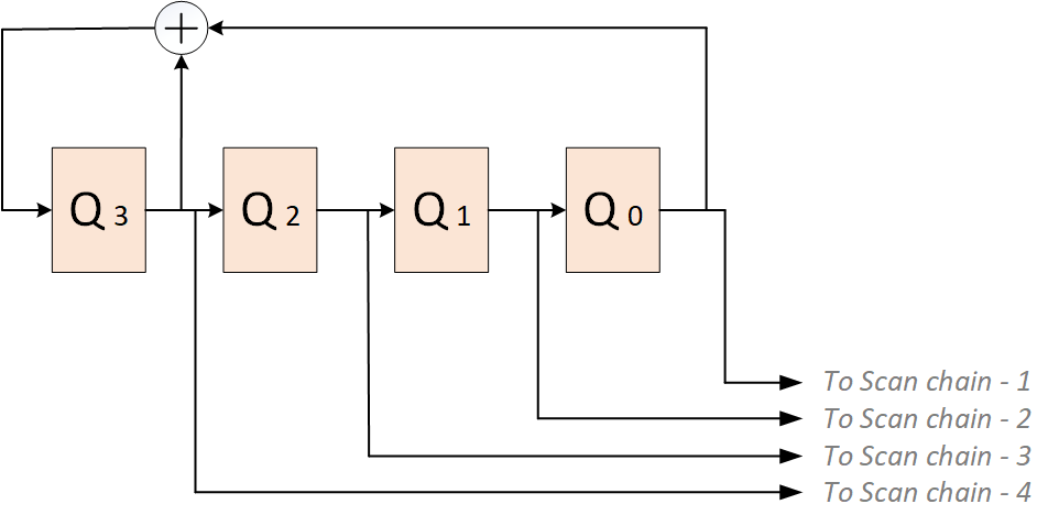
It generates the test patterns required to sensitize the faults and propagate the effect to the outputs (of the CUT). Typically a Standard form LFSR is used for generating pseudo random patterns which acts as the input test vector. Each flop in the LFSR feeds a scan chain as shown in the Figure 2. In pseudo random patterns, the patterns are repeated after certain interval of time, which is why we use the term ‘pseudo’.
As discussed earlier, the LFSR is represented by its characteristics polynomial. Suppose we are initializing two 4-degree LFSR having characteristics polynomial f(x) = x4 + x3 +1 and f(x) = x4 + x2 + 1, with 1000.

The sequence generated by the LFSR with characteristics polynomial f(x) = x4 + x3 +1 repeats itself after 15 sequences, thus has a period of 24 – 1 = 15. But the sequence generated by the LFSR with characteristics polynomial f(x) = x4 + x2 +1 repeats itself after 6 sequences.
If the sequence generated by the LFSR has a period 2N – 1, where N = number of flops in LFSR (or degree of the LFSR), then the LFSR is called maximum-length sequence or m-sequence.
Now the characteristic polynomial of the m-sequence LFSR is called primitive polynomial.
Note: Primitive polynomial is not unique for a given ‘N’ degree LFSR.
Example – x4 + x3 +1 and x4 + x +1 both are primitive polynomial of 4-degree LFSR.
The choice of polynomial has a great impact on the cycle length. Better the length of cycle implies better TPG, thus a LFSR implementing a primitive polynomial is best suited for Test Pattern Generation.
Why we need Phase Shifter?
One of the major disadvantage of LFSR is there is not enough randomness. Consider the same m-sequence LFSR we discussed earlier f(x) = x4 + x3 +1. As shown in Figure 4, in the absence of phase shifter, there exists a diagonal relationship between adjacent bit stream.
To introduce more randomness between the bit streams, we use a phase shifter which is implemented by XOR network. Basically each bit stream is phase shifted by some cycles. As we can see in the presence of phase shifter, the diagonal relationship no longer exists. More randomness helps in increasing the fault coverage. Also as we can see in the example, the 4-degree LFSR is feeding 5 scan chains. Thus LFSR with phase shifter can support more scan chains (typically a ‘N’ degree LFSR can support maximum of ‘N’ scan chains without phase shifter).

(Check the color coding of the bits to understand how phase shifting works)
How to find the seed of a LFSR?
Here we will discuss about how to find the initial state of the LFSR (or seed) with a given LFSR and test pattern. Consider a simple example shown below.

The LFSR feeds a scan chains with 10 flops. S0-S9 are the test pattern specified by the ATPG and Q0-Q3 are the seeds of the LFSR.
There are two methods –
1. Cycle by cycle tracing
2. System of Linear equations
We will only discuss about the solving by system of linear equations. We can model the above scenario in a system of linear equations.
Note: S0-S9 values will be loaded to the chain serially such that S9 will be loaded first to the chain in the 1st clock cycle and then will be shifted to the right in the next clock cycle and simultaneously S8 will be loaded to the chain. This continues for 10 clock cycles till all the values are loaded at its required position.
Initial conditions (S9 is the first input to the chain from LFSR, thus equal to Q0, and similarly till S6) –
S9 = Q0
S8 = Q1
S7 = Q2
S6 = Q3

Note: ⊕ = XOR
S5 = S9 ⊕ S6 = Q3 ⊕ Q0 = Q0 ⊕ Q3
S4 = S8 ⊕ S5 = Q1 ⊕ Q3 ⊕ Q0 = Q0 ⊕ Q1 ⊕ Q3
S3 = S7 ⊕ S4 = Q2 ⊕ Q1 ⊕ Q3 ⊕ Q0 = Q0 ⊕ Q1 ⊕ Q2 ⊕ Q3
S2 = S6 ⊕ S3 = Q3 ⊕ Q3 ⊕ Q1 ⊕ Q2 ⊕ Q0 = Q0 ⊕ Q1 ⊕ Q2
S1 = S5 ⊕ S2 = Q3 ⊕ Q0 ⊕ Q1 ⊕ Q2 ⊕ Q0 = Q1 ⊕ Q2 ⊕ Q3
S0 = S4 ⊕ S1 = Q1 ⊕ Q3 ⊕ Q0 ⊕ Q1 ⊕ Q2 ⊕ Q3 = Q0 ⊕ Q2
Thus we have 10 equations and 4 variables Q0, Q1, Q2 and Q3.
Suppose the pattern S0 S1 S2 S3 S4 S5 S6 S7 S8 S9 is: 1 X X X 0 1 X X 1 0 respectively.
Then we write the 10 equations in the form of matrix as shown below –
From the matrix –
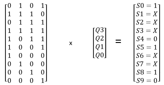
S9 = Q0 = 0
S8 = Q1 = 1
S5 = Q0 ⊕ Q3 = 1, but Q0 = 0, thus Q3 = 1
S6 = Q2 ⊕ Q0 = 1, but Q0 = 0, thus Q2 = 1
Thus the required seed of the LFSR is 1110
Note: The system of linear equations are not always solvable, in that case we cannot load that particular pattern and thus will not be able to cover faults targeted by that pattern. The number of variables depends upon the LFSR degree, more variable implies the probability of getting a solution increases.
LFSR degree?
Suppose we have a ‘N’ degree LFSR that needs to load a pattern having ‘S’ number of care bits, then we have ‘N’ variables and ‘S’ equations to solve. Example – if the pattern is 1 X X X 0 1 X X 1 0, then ‘S’ = 5.
Now, what is the minimum ‘N’ needed to guarantee a solution (or seed) can be found for the given pattern?
Well, study shows that the probability of not finding a solution is 10-6 (which is very less) when N ≥ (S+20).
