


1. Introduction
A surge-type glacier experiences quasi-periodic cyclical variations between long periods of slow flow during the quiescent phase, followed by shorter periods of considerably faster flow during the active phase of a surge. Ice motion during the active phase is typically 10–1000 times faster than during the quiescent phase (Murray and others, Reference Murray, Strozzi, Luckman, Jiskoot and Christakos2003). While surge-type glaciers represent approximately 1% of all glaciers worldwide, they have been found to cluster within particular regions, including the Canadian Arctic (Sevestre and Benn, Reference Sevestre and Benn2015). The first systematic inventory of surge-type glaciers in the Canadian Arctic Archipelago (CAA: Ellesmere, Axel Heiberg, and Devon islands) compiled by Copland and others (Reference Copland, Sharp and Dowdeswell2003) revealed 51 surge-type glaciers, of which most are large tidewater glaciers. More recent studies have identified additional surge-type glaciers (e.g., Van Wychen and others, Reference Van Wychen2016, Reference Van Wychen, Hallé, Copland and Gray2022), and Sevestre and Benn (Reference Sevestre and Benn2015) state that 54 (0.46%) of the 11 757 glaciers in the Canadian Arctic at that time were classified as surge-type. The cold and dry climate of the Canadian Arctic falls outside of the optimal climatic envelope for surging suggested by Sevestre and Benn (Reference Sevestre and Benn2015), so there are fewer surge-type glaciers than in some other locations, such as Svalbard. However, surge-type glaciers in the CAA tend to be larger than average (Copland and others, Reference Copland, Sharp and Dowdeswell2003; Sevestre and Benn, Reference Sevestre and Benn2015), and therefore occupy a proportionally larger part of the landscape than their count would suggest.
The greatest terminus advances of surge-type glaciers inventoried by Copland and others (Reference Copland, Sharp and Dowdeswell2003) occurred on western Axel Heiberg Island, where Airdrop, Iceberg and Good Friday glaciers advanced by approximately 4.5, 5, and 7 km, respectively, over the 40-year period from 1959 to 1999. Out of 13 glaciers with signs of unstable flow on Axel Heiberg Island, these three large glaciers were the only confirmed surge-type glaciers. While a detailed analysis of the dynamics of Good Friday was undertaken by Medrzycka and others (Reference Medrzycka, Copland, Van Wychen and Burgess2019), showing that the glacier has been continuously advancing for at least the last 70 years, the long-term changes in terminus position, velocity, and ice thickness of Iceberg Glacier remains largely unknown.
In this study, we reconstruct the surge history of Iceberg Glacier from 1950 to 2021 using a variety of remotely sensed data, including historical aerial photographs, declassified intelligence satellite photographs, optical satellite imagery and synthetic aperture radar (SAR) data. The terminus positions of Iceberg Glacier from the 1950s to present are combined with changes in ice surface velocities and surface elevation to elucidate its surge behaviour over the past ~70 years. Studies of surge-type glaciers in the Canadian Arctic remain sparse (e.g., Copland and others, Reference Copland, Sharp and Dowdeswell2003; Short and Gray, Reference Short and Gray2005; Medrzycka and others, Reference Medrzycka, Copland, Van Wychen and Burgess2019; Van Wychen and others, Reference Van Wychen2021, Reference Van Wychen, Hallé, Copland and Gray2022), in part due to a lack of detailed observations through an entire quiescent-active-quiescent cycle. We have been able to collate data to provide such an insight for the first time and use it to undertake an analysis of the surge characteristics of Iceberg Glacier, including the length and dynamics of its active phase.
2. Study site
Axel Heiberg Island, located in the northern CAA (Fig. 1), has a total land area of ~43 000 km2 and a glacierised area of ~11 700 km2 contained within >1100 glaciers (Ommanney, Reference Ommanney1969; Thomson and others, Reference Thomson, Osinski and Ommanney2011). The island is home to two major ice caps: Müller Ice Cap located in the north, and Steacie Ice Cap in the south (Ommanney, Reference Ommanney1969). This region has mean annual air temperatures of approximately −20°C and mean annual precipitation ranging from 58 mm a−1 water equivalent at sea level measured at Eureka, 100 km to the east (Fig. 1), to 370 mm a−1 water equivalent at an elevation of 2120 m above sea level (a.s.l.) (Cogley and others, Reference Cogley, Adams, Ecclestone, Jung-Rothenhäusler and Ommanney1996; Thomson and others, Reference Thomson, Zemp, Copland, Cogley and Ecclestone2017).

Fig. 1. (a) Location of Iceberg Glacier, Airdrop Glacier and Good Friday Glacier on Axel Heiberg Island, Nunavut, in the CAA. (b) The centerline of Iceberg Glacier (red line), with numbers indicating 5 km distance markers starting from the maximum terminus position in 1997. Base image: Landsat 8, 12 August 2020. Data: Statistics Canada, 2016 Census. Provinces/territories – Cartographic Boundary File (https://www12.statcan.gc.ca/census-recensement/2011/geo/bound-limit/bound-limit-2016-eng.cfm). Natural Resources Canada. Lakes, Rivers and Glaciers in Canada – CanVec Series – Hydrographic Features (https://open.canada.ca/data/en/dataset/9d96e8c9-22fe-4ad2-b5e8-94a6991b744b).
Iceberg Glacier (79.60°N, 92.19°W) is a large tidewater surge-type glacier that drains the west side of Müller Ice Cap (Fig. 1). It has a total basin size of ~1000 km2 and a main trunk length of ~35 km (Van Wychen and others, Reference Van Wychen2016), making it significantly larger than the average surge-type glacier area of 627 km2 in the Canadian Arctic (Sevestre and Benn, Reference Sevestre and Benn2015). Iceberg Glacier has been observed in both active and quiescent phases of the surge cycle, the only such glacier out of the three observed surge-type glaciers on western Axel Heiberg Island (Van Wychen and others, Reference Van Wychen2016; Medrzycka and others, Reference Medrzycka, Copland, Van Wychen and Burgess2019).
Although knowledge of the dynamics of Iceberg Glacier remain limited, the glacier has been referred to in a handful of papers. It was first deemed to show evidence of a past surge by Ommanney (Reference Ommanney1969), who reported that in 1959, the glacier was stagnant, its terminus showed retreat characteristics, and extensive potholing of the ice surface extended to at least 10 km up-glacier from its terminus, suggesting that the glacier was in its quiescent phase. By 1992 the glacier had advanced by ~3.5 km, followed by a further advance of ~1.5 km from 1992 to 1999 (Copland and others, Reference Copland, Sharp and Dowdeswell2003). In total, Iceberg Glacier underwent a 21.5 km2 increase in area from 1959 to 2000 (Thomson and others, Reference Thomson, Osinski and Ommanney2011). Both 1992 and 1999 satellite imagery reveal intense crevassing and large looped moraines across the lower glacier, with manual tracking of surface features indicating motion of ~4 km between these dates, equivalent to a mean velocity of ~575 m a−1 (Copland and others, Reference Copland, Sharp and Dowdeswell2003). Subsequently, the glacier was flowing more slowly in the fall of 2000, but maintained a flow rate of 75–130 m a−1 over its lower 15 km, followed by a drop to <25 m a−1 by midwinter 2004 (Short and Gray, Reference Short and Gray2005). The ensuing slowdown started at the terminus and propagated up-glacier until approximately 2010, when the entire glacier trunk became essentially stagnant (Van Wychen and others, Reference Van Wychen2016). This slowdown was coincident with a terminus retreat of ~1.5–2.5 km between 2000 and 2014, and a decrease in dynamic discharge from 0.03 Gt a−1 in 2000 to 0.00 Gt a−1 from 2001 to 2015 (Van Wychen and others, Reference Van Wychen2016). Preliminary evidence from these studies suggests that Iceberg Glacier has an active phase between 10 and 30 years (Medrzycka and others, Reference Medrzycka, Copland, Van Wychen and Burgess2019).
3. Methods
3.1 Terminus position
The terminus extents of Iceberg Glacier were digitised for the period 1959–2021 using 42 air photos and satellite images (Table 1). The 1959 terminus position was mapped from a nadir aerial photograph taken at an altitude of ~9000 m a.s.l. by the Royal Canadian Air Force (RCAF). This image was acquired from the National Air Photo Library, Ottawa, Canada. The 1966 terminus outline was mapped from a declassified image from the KH-4 Corona reconnaissance satellite missions, acquired from the United States Geological Survey (USGS). The scanned historical aerial photographs and declassified intelligence satellite photos were cropped to cover only the terminus region of Iceberg Glacier and then manually georeferenced using a first order polynomial (affine) transformation and a minimum of 8 tie points in ArcGIS 10.8.1. The terminus positions were then manually outlined in ArcMap.
Table 1. Imagery used for mapping the terminus positions of Iceberg Glacier in this study
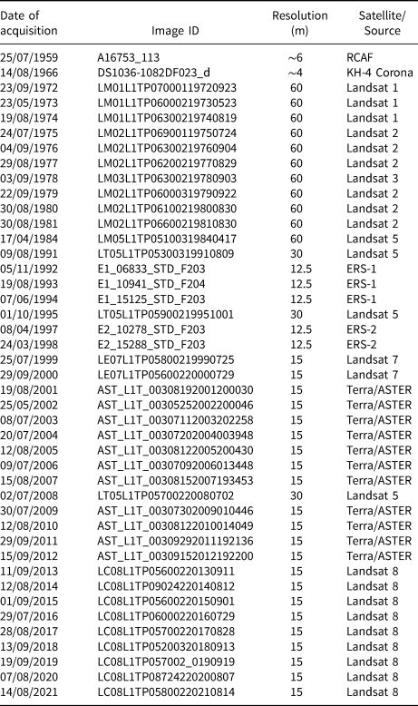
All of the terminus positions from 1972 to 2021 were delineated using satellite imagery. European Remote-Sensing Satellite (ERS) SAR data from the 1990s was obtained from the Alaska Satellite Facility (ASF; https://search.asf.alaska.edu). These scenes were downloaded in Level 1 (i.e., processed) format and geocoded with the ASF MapReady software. However, some of these scenes were poorly georeferenced and had to be manually adjusted using the Shift tool from the Georeferencing toolbar in ArcGIS to properly align the imagery with recent Landsat 8 scenes. Optical satellite imagery since the 1970s was used from Landsat 1–8, acquired from the USGS Earth Explorer data portal (http://earthexplorer.usgs.gov) in Level 1TP (L1TP; precision and terrain corrected) format. Landsat data products required no pre-processing since L1TP scenes are orthorectified and geometrically/radiometrically corrected. Advanced Spaceborne Thermal Emission and Reflection Radiometer (ASTER) L1T optical satellite scenes were acquired from USGS Earth Explorer, NASA's Earthdata search (https://search.earthdata.nasa.gov/search) and the METI AIST Data Archive System (https://gbank.gsj.jp/madas/map/index.html). When possible, late summer (July–September) images were selected to ensure minimal snow cover and sea ice. No cloud-free images were available for 1982–91 other than a single Landsat 5 scene providing partial coverage of the terminus of Iceberg Glacier (Table 1), resulting in a data gap during that period.
Once all the outlines were completed, the Glacier Termini Change Tracking (GTT) toolbox from Urbanski (Reference Urbanski2018) was used to help determine the mean changes in terminus-wide position between each year. The GTT toolbox uses a computational geometry algorithm to perform a 2-D analysis of terminus position changes over time. Total and mean yearly change rates in terminus positions were subsequently quantified for specific periods based on image availability and stages of the surge cycle. A conservative estimate of the maximum uncertainty resulting from the manual delineation of the terminus positions is 2 pixels (Kochtitzky and others, Reference Kochtitzky2019), which we use instead of the more usual 1 pixel error (Paul and others, Reference Paul2013), to allow for variations in the georeferencing and orthorectification accuracy of the satellite imagery. This equates to 120 m for Landsat 1–3, 60 m for Landsat 4–5, 30 m for Landsat 7–8, 25 m for ERS-1/2, ~12 m for the 1959 historical aerial photograph and ~8 m for the KH-4 image. Assuming that uncertainties are independent (i.e., caused by random error) and there is no systematic bias, uncertainties for the terminus advance/retreat rate of Iceberg Glacier over the different time periods were calculated from:

However, the manual georeferencing of the 1959 historical aerial photograph and 1966 KH-4 Corona image introduced additional uncertainty in the glacier terminus position changes calculated from these images. Comparison of fixed bedrock features near to the glacier terminus indicate an offset of ~40 m between the 1959 historical aerial photograph and the 1966 KH-4 image and an offset of ~50 m between the 1966 KH-4 image and the 1972 Landsat 1 image. These offsets were added to the numerator of Eqn 1.
3.2 Ice velocities
3.2.1 Feature tracking
Ice surface velocities from 1972 to 1981 were derived from Landsat 1–3 optical satellite imagery using the Glacier Image Velocimetry (GIV) app (Van Wyk de Vries, Reference Van Wyk de Vries2021a, Reference Van Wyk de Vries2021b). GIV enables rapid determination of velocities based on a feature-tracking algorithm which matches persistent irregularities on the ice surface between images, which, over time, translate to surface velocity (Van Wyk de Vries and Wyckert, Reference Van Wyk de Vries and Wickert2021). Velocities were derived from near-annually separated Landsat 1–3 images with the same orbital geometry (i.e., same path and row number) that were subset to a smaller area covering only Iceberg Glacier and its immediate surroundings. Some of the early Landsat images are somewhat poorly georeferenced, so a few Landsat 1–3 images had to be manually shifted, as described in section 3.1. This was to ensure that the two images in each pair overlaid each other properly, which helps minimise errors in the resulting velocities.
Subsequently, the velocity data for Iceberg Glacier were filtered based on flow direction. The glacier was separated into two parts where the glacier changes flow direction from approximately SSE to SSW at about 18 km from the terminus, just above the junction between the lowermost tributary and the trunk (Fig. 1). To account for differences in the flow direction between these two areas, the lower part and the upper part of the glacier were filtered using different values. Cells with a flow direction outside of the range of 150–295° for the lower part of Iceberg Glacier and 100–265° for the upper part of the glacier were excluded to help filter out false matches. These ranges were chosen to account for roughly 45° in variability relative to the orientation of the centreline in a downstream direction and for the ice flow at the junctions between tributaries and trunk. The filtering was undertaken using Raster Calculator in ArcGIS to exclude flow direction cells outside of the specified value range for each part of the glacier, and the Extract by Mask tool was then used to mask the velocity map to the extent of the filtered flow direction map. Automated velocity mapping with Landsat 1–3 imagery can yield relatively large uncertainties (Table 2) and incomplete coverage, hence the per-cell mean value for the velocity rasters from 1972 to 1980 was computed to reduce errors and provide complete coverage of the glacier surface. This gives an estimate of the pre-surge velocities.
Table 2. Landsat (L) and ERS scenes used to derive ice surface velocities, with associated uncertainty quantified by the velocities captured over nonglacierised terrain
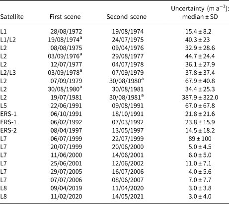
a Scenes that were manually shifted in ArcMap.
3.2.2 GAMMA InSAR
Velocities were derived from ERS-1/2 SAR data for the years 1991, 1992, and 1997. The raw SAR data were downloaded from the ASF website as Level 0 products. Scene pairs with the same orbital geometry (i.e., same path and frame) and a time separation of 12–35 days were acquired. The raw data were then converted to Single Look Complex (SLC) to generate the files required for the computation of displacements using interferometric SAR (InSAR) processing within GAMMA Remote Sensing software& nbsp;(Werner and others, Reference Werner, Wegmüller, Strozzi and Wiesmann2000), which enables processing of raw SAR data to end products, such as DEMs or glacier velocity maps. The GAMMA Modular SAR Processor (MSP) was used to calculate SLC and multi-look intensity images in radar range-Doppler coordinates from the raw data. Next, GAMMA Interferometric SAR Processor (ISP) uses these files to compute displacements between pairs of SAR scenes. The second image was first resampled into the geometry of the first image in order to co-register the two SLCs based on orbital data and terrain height data from the Copernicus DEM. Next, the orbital data were used to determine the offset between the two images, which is refined with a 2-D cross-correlation analysis. Range and azimuth displacements between the two images were then estimated with a cross-correlation optimisation. A patch size of 160–192 range pixels by 320–384 azimuth pixels and a step size of 24 range pixels by 48 azimuth pixels were used for each image pair.
Subsequently, the displacements were converted from RADAR geometry to metres in ground range and from complex to real numbers. The ASTER GDEM version 3 was used to create a look-up table between the displacements and the DEM file, which was applied to add the georeferencing information to the centre of every matching window used to calculate the displacements. GeoTIFF files of the outputs were then created and the total displacement between the two images was computed from:

In order to convert the total displacement to metres per year, the values were divided by the total number of days between the two images to calculate the daily displacements, which was then multiplied by 365.25 to compute the annual displacements. This facilitates comparison between the velocities derived with GIV and the ones acquired from the NASA ITS_LIVE dataset, which are already standardised to annual values.
3.2.3 NASA ITS_LIVE
All surface velocities since 1999 were acquired from NASA's Inter-mission Time Series of Land Ice Velocity and Elevation (ITS_LIVE; https://nsidc.org/apps/itslive/) dataset, which provides a near-global record of glacier velocities at high temporal resolution from optical satellite imagery (Gardner and others, Reference Gardner, Fahnestock and Scambos2019). The data were generated using the autonomous Repeat Image Feature Tracking (auto-RIFT v0.1) processing scheme produced by the NASA Jet Propulsion Laboratory (Gardner and others, Reference Gardner2018), with imagery mainly from Landsat 4, 5, 7, and 8. The velocity data have a spatial resolution of 120 or 240 m and can be gathered from the data portal either as scene-pair velocities with a time separation ranging from 6 to 546 days, or as monthly or annual velocity mosaics created from the synthesis of all scene-pair velocities.
The regional composite of annual mean surface velocities for Arctic Canada North for 2000–18 was downloaded and subset to Axel Heiberg Island in QGIS 3.6. Some of the velocity mosaics from 2000 to 2008 provide no or partial coverage of Iceberg Glacier, thus scene-pair velocities were downloaded to fill in the gaps during that period. Additionally, scene-pair velocities provided coverage for 1991, 1999, 2019, 2020, and 2021. For years with many available image-pair velocities (i.e., >150) for the area of interest, the data products were filtered by setting a minimum time separation between the two images (i.e., >60 days) and/or a minimum coverage (i.e., the percentage of possible glacier pixels that have reported velocities) of between 10 and 90 per cent, depending on the amount of data available for a given year. After gathering all velocity products for a given year, each velocity file was inspected to keep the scene-pair velocities with the highest coverage over Iceberg Glacier and with the smallest apparent errors (i.e., the lowest velocities over bedrock; Table 2). GeoTIFF files of the velocity errors for the annual mosaics for the period 2000–18 were downloaded. All GeoTIFF files (i.e., velocities and errors) were projected to NAD 1983 UTM Zone 15N.
Uncertainty estimates for all of the scene-pair data from GIV, GAMMA and ITS_LIVE were determined by computing the median and SD velocity over nonglacierised terrain surrounding Iceberg Glacier (Table 2; Fig. 2d). The median value was used instead of the mean to provide a better measure of central tendency of the uncertainties due to the presence of outliers in the data. For the velocity mosaics, the median yearly error value over Iceberg Glacier from the ITS_LIVE GeoTIFF annual error files (i.e., v_err) was calculated and used to estimate uncertainties (see http://its-live-data.jpl.nasa.gov.s3.amazonaws.com/documentation/ITS_LIVE-Regional-Glacier-and-Ice-Sheet-Surface-Velocities.pdf for an explanation of how errors were quantified for the annual mosaics).
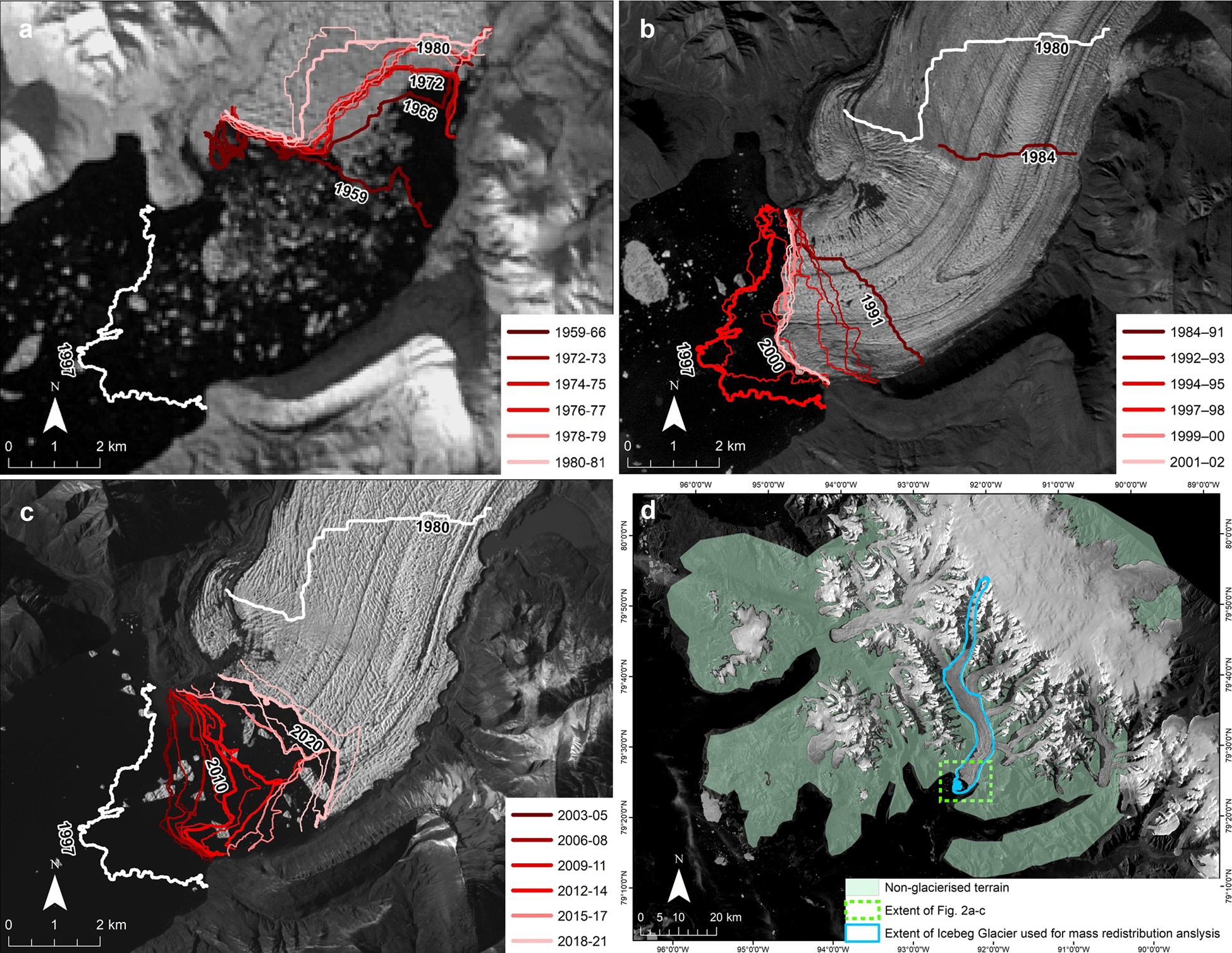
Fig. 2. Terminus positions of Iceberg Glacier for: (a) 1959–81 (pre-surge), (b) 1984–2002 (surge) and (c) 2003–21 (post-surge). The colour palette ranges from dark red (earliest) to light pink (latest) while certain years are annotated and their respective terminus lines are thicker to help with visual interpretation. The pre-surge (1980) and maximum surge (1997) terminus positions are included in each plot for reference. (d) Distribution of nonglacierised terrain used for the computation of off-ice uncertainties for ice velocity and elevation change data and the extent over which the mass redistribution analysis (Section 5.1) was undertaken. Base images: (a) Landsat 2, 30 August 1981, (b) Landsat 7, 25 July 1999, (c) Landsat 8, 7 August 2020, (d) Landsat 8, 10 August 2020.
3.3 Surface elevation
3.3.1 sPyMicMac
A pair of July 1977 KH-9 Hexagon declassified intelligence satellite photos (image ID: DZB1213-500054L001001 and DZB1213-500054L002001) and 18 historical air photographs (photos 098–115 from roll A16754) taken over Iceberg Glacier in July 1959 were used to create DEMs with sPyMicMac (McNabb and others, Reference McNabb, Girod, Nuth and Kääb2020; https://spymicmac.readthedocs.io), a set of Python tools for processing historical spy satellite and aerial imagery using the MicMac photogrammetric software for 3D reconstruction (Rupnik and others, Reference Rupnik, Daakir and Pierrot Deseilligny2017). This enables glacier surface elevations and volume changes to be computed for early periods, as most global estimates of glacier volume changes are only available since the year 2000 (Zemp and others, Reference Zemp2019; Hugonnet and others, Reference Hugonnet2021).
Although the general workflow is virtually identical for both KH-9 and historical aerial photographs, which were processed separately, the pre-processing steps differ slightly. Pre-processing of the KH-9 data consisted of joining the two halves of both photographs together since KH-9 images are scanned into two parts (e.g., DZB1213-500054L001001_a and DZB1213-500054L001001_b) because of the large size of the film of ~9″ × 18″, and resampling the two images to correct distortions in the film (e.g., Maurer and Rupper, Reference Maurer and Rupper2015). The resampling is based on the location of the Reseau markers in KH-9 images, which sPyMicMac automatically finds and resamples to their expected location. The next step consisted of removing the Reseau markers from the KH-9 images and joining the two slightly overlapping image halves together. Since the KH-9 images were relatively low contrast, contrast enhancement was undertaken using one of sPyMicMac's functions, which processes the images with a median filter to reduce noise and applies a linear contrast stretch as well as gamma adjustment.
For the pre-processing of historical air photos, the same contrast enhancement was applied to each image, although no de-striping or de-noising, which can help remove artefacts occasionally found in aerial photos, was necessary. While this is done automatically when processing KH-9 images, some processing files, such as files containing information on the dimension of the images, the focal length of the camera used, and the location of the fiducial markers in the image geometry, had to be created. Next, the images were resampled to a common geometry using the four fiducial markers found in the corners of the historical air photos, each of which had to be precisely located in all of the 12 images.
Once the KH-9 images and historical air photos were resampled, tie points were computed by matching all pairs of images (i.e., one pair for the KH-9 images and several for the air photos), and these were then used, along with a basic radial distortion model, to estimate the relative orientation of each image (McNabb and others, Reference McNabb, Girod, Nuth and Kääb2020). Thereafter, the relative (i.e., not georeferenced) orthoimages and DEM were generated using the orientation files from the previous step and a relative orthomosaic was created from the individual orthoimages. Before georeferencing the relative orthomosaic and DEM, a number of files were used to automatically find control points and to estimate and iteratively refine the absolute orientation. These files included a 2020 Sentinel-2 mosaic used as the reference orthoimage, the ASTER GDEM used as the reference DEM, image footprints from USGS for the KH-9 scenes or from NAPL for the 1959 air photos, and a modified version of the Randolph Glacier Inventory (RGI) 6.0 glacier outlines (Pfeffer and others, Reference Pfeffer2014) used as an exclusion mask to avoid searching for matches over glaciers or the ocean/sea ice. Finally, the orientation files and control points were used to generate the absolute (i.e., georeferenced) orthomosaic and DEM.
3.3.2 MMASTER
DEMs were generated for the years 2000–21 from ASTER imagery using MicMac ASTER (MMASTER; Girod and others, Reference Girod, Nuth, Kääb, McNabb and Galland2017; Table 3). Since 1999, ASTER has collected 15 m resolution stereo images, which have been used to produce the ASTER GDEM (Global Digital Elevation Model) at 30 m grid spacing (https://asterweb.jpl.nasa.gov/gdem.asp). However, the dates of individual elevations in the ASTER GDEM are unknown, and noise is present in the satellite data in the form of ‘jitter’ (i.e., uncorrected errors in the imagery geometry due to sensor motion), which can result in anomalies and artefacts (Girod and others, Reference Girod, Nuth, Kääb, McNabb and Galland2017).
Table 3. Mean total changes and mean change rates of the terminus position of Iceberg Glacier for different periods from 1959 to 2021.
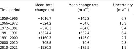
*Negative values indicate a terminus retreat, while positive values indicate a terminus advance.
The MMASTER software package was used to produce DEMs from ASTER stereo satellite imagery with reduced overall noise and fewer unmatched areas compared to NASA's standard AST14DMO product, with a horizontal resolution of 30 m or less and a vertical uncertainty of 10 m (Girod and others, Reference Girod, Nuth, Kääb, McNabb and Galland2017). A total of 816 ASTER L1A scenes (i.e., reconstructed unprocessed instrument data) were downloaded from NASA's Earthdata Search portal (https://search.earthdata.nasa.gov) for the area of interest using a cloud filter to exclude scenes with a cloud cover greater than 80%. Subsequently, batch processing of the MMASTER workflow was conducted on the Cedar supercomputer from Compute Canada (https://docs.computecanada.ca/wiki/Cedar) to create 816 DEMs from the raw ASTER L1A products. The DEMs were then visually inspected to exclude those with large amounts of noise resulting from cloud cover or otherwise poor coverage of Iceberg Glacier and its tributaries. The DEMs provided relatively good temporal coverage over the period 2000–21, although no good quality data were available over Iceberg Glacier for 2000, 2008 and 2015, while others years, such as 2010, 2011, 2020, and 2021 did not have complete coverage.
3.3.3 Co-registration and trend analysis
All DEMs created with sPyMicMac and MMASTER were iteratively co-registered using a DEM co-registration script from the pybob Python package (https://github.com/iamdonovan/pybob), based on the co-registration algorithm described by Nuth and Kääb (Reference Nuth and Kääb2011), which removes shifts between DEMs and checks for elevation dependant and sensor-specific biases. Post-processing of the ASTER DEMs included spatial and temporal filtering of outliers from each DEM by excluding pixels that had a difference from the ASTER GDEM greater than a specified threshold value. Difference maps between each DEM from 2003 to 2021 and the ASTER GDEM were computed and visually inspected to determine an appropriate threshold to differentiate real elevation changes on the glacier surface from noise due to cloud cover or other biases for 6-year periods (i.e., 2003–09, 2009–15 and 2015–21). Different threshold values were used for the terminus compared to the rest of the glacier since elevation changes were consistently greatest at the terminus region. Threshold elevation changes for the terminus area of Iceberg Glacier ranged from 70 to 100 m, while thresholds for the rest of the glacier were between 35 and 65 m. This spatial and temporal filtering of outliers was automated using models created with ModelBuilder in ArcGIS. The use of overlapping DEMs from within the same year was avoided to minimise the computation of false trends arising from vertical uncertainties, which are exacerbated when the time separation between two DEMs is short.
Finally, the make_stack.py Python script from the pygeotools Python package (https://github.com/dshean/pygeotools) was used to compute the trend in elevation changes for Iceberg Glacier from the ASTER DEMs for the 6-year periods 2003–09, 2009–15, 2015–21 as well as for 2003–21. This script computes various statistics (e.g., min, max, mean, trend) using a raster time series object (i.e., a stack of input rasters) from which a linear regression is calculated. When the temporal coverage of DEMs is sufficient, such as for these time periods, computing the trend in elevation changes between multiple DEMs using make_stack.py yields lower uncertainties than differencing just one DEM from another.
For the 1959 and 1977 DEMs created with sPyMicMac, elevation changes were computed by calculating the difference between two DEMs using the Minus tool in ArcGIS, which subtracts the value of the second input raster from the value of the first input raster on a cell-by-cell basis. Elevation changes were determined between 27 July 1959 (air photographs) and 13 July 1977 (KH-9) and between 13 July 1977 and an ASTER DEM mosaic from 26 May and 28 May 2003. The 2003 DEM was used instead of the one from 20 May 2001 to include surge termination, which occurred in 2003. This way, the 1977–2003 DEM differencing approximately coincides with the active phase of the surge. Elevation trends were then standardised to annual values by dividing the result by the number of years elapsed between the two DEMs.
To minimise noise from individual grid cells, plots of the results were made showing the average change in elevation across the glacier surface for each 10 m elevation bin based on the 2001–21 mean elevation of the glacier computed from all the available ASTER DEMs. Uncertainties in the trends and DEM differencing results were determined by calculating the median absolute value over stable (i.e., nonglacierised) terrain (Fig. 2d).
4. Results
4.1 Terminus position changes, surge initiation and termination
Historical air photographs, spy satellite imagery and Landsat 1–3 scenes show that the terminus of Iceberg Glacier was retreating from 1950 to 1981. The glacier front underwent a ~1.9 km mean terminus-wide retreat in 22 years between 1959 and 1981 at a mean rate of −145.2 ± 6.7 m a−1 for the period 1959–66, −54 ± 15.9 m a−1 for 1966–72, and −64 ± 9.4 m a−1 for 1972–81 (Fig 2a; Table 3). This retreat was especially pronounced over the eastern side of the terminus, while the westernmost ~2 km of the terminus saw very little change. Subsequently, Iceberg Glacier experienced a pronounced terminus advance of approximately 5.3 km from 1981 to 1991, at a mean rate of 532.4 ± 6.4 m a−1 during those ten years (Fig. 2b; Table 3). In addition, a Landsat 5 scene from 1984 with partial coverage of the terminus of Iceberg Glacier shows that the eastern half of the terminus advanced by about 2.3 km between 1981 and 1984 at a mean rate of >750 ± 42.4 m a−1 (Fig. 2b; Table 3). This indicates that Iceberg Glacier was likely surging in 1984. A further advance of ~1.2 km followed from 1991 to 2000, which occurred at a mean rate of 145 ± 2.7 m a−1 (Fig. 2b; Table 3). The glacier reached its maximum observed surge extent in the winter of 1997 at a distance of ~7.6 km from its 1981 position, with parts of the terminus having advanced by more than 10 km.
The terminus positions from 1991 to 2000 were digitised from a combination of summer optical satellite imagery (1991, 1995, 1999 and 2000) and winter ERS-1 and ERS-2 SAR scenes (1992, 1993, 1994, 1997, and 1998). The winter ERS scenes show that as the ice front pushed forward, it frequently splayed out into the adjacent sea ice, forming a digitate terminus that later would break apart once the sea ice started retreating from Iceberg Bay during the following summer months. These seasonal fluctuations make it more challenging to determine the temporal evolution of the terminus extent during the active phase of the surge. However, it appears that Iceberg Glacier reached its maximum terminus position in 1996–97 since the terminus was less extensive in the winter of 1995, 1998, and 1999.
In 2000–10, which marks the transition from the active phase to the quiescent phase of the surge cycle, the terminus of Iceberg Glacier retreated by about 0.7 km at a mean rate of 70.6 ± 2.3 m a−1. The ice front then started retreating at an accelerated pace of 175.5 ± 1.9 m a−1 from 2010 to 2021, equating to a total retreat of ~1.9 km over approximately the last decade (Fig. 2c; Table 3). A large calving event occurred between 12 August 2014 and 1 September 2015, resulting in a terminus retreat of up to ~1 km (average of 432 m across the terminus width) and a loss of >2 km2 of ice.
On average, Iceberg Glacier retreated by >2 km between 1950 and 1980, followed by a ~6.5 km advance from 1981 to 2002 during the active phase, and a >2.5 km retreat since the glacier became quiescent in 2003. These results are in line with observations made by Copland and others (Reference Copland, Sharp and Dowdeswell2003) and Van Wychen and others (Reference Van Wychen2016), who reported a terminus advance of ~5 km from 1959 to 1999 followed by a retreat of ~1.5–2.5 km from 2000 to 2014.
High-resolution historical aerial photographs from 1950 and 1959 reveal that the surface of Iceberg Glacier was heavily potholed (Fig. 3a). Spy satellite imagery from 1966 and 1977 also show potholing, although it was less extensive than in the 1950s. This observation, along with the retreating terminus during that period suggests that the glacier was in its quiescent phase of the surge cycle and had previously surged. Distorted medial moraines located at the intersection of the lower two tributaries and the glacier trunk (Fig. 3b) from 1959 to 1981 indicate that they are subject to irregular ice flow and could have surged in the past.
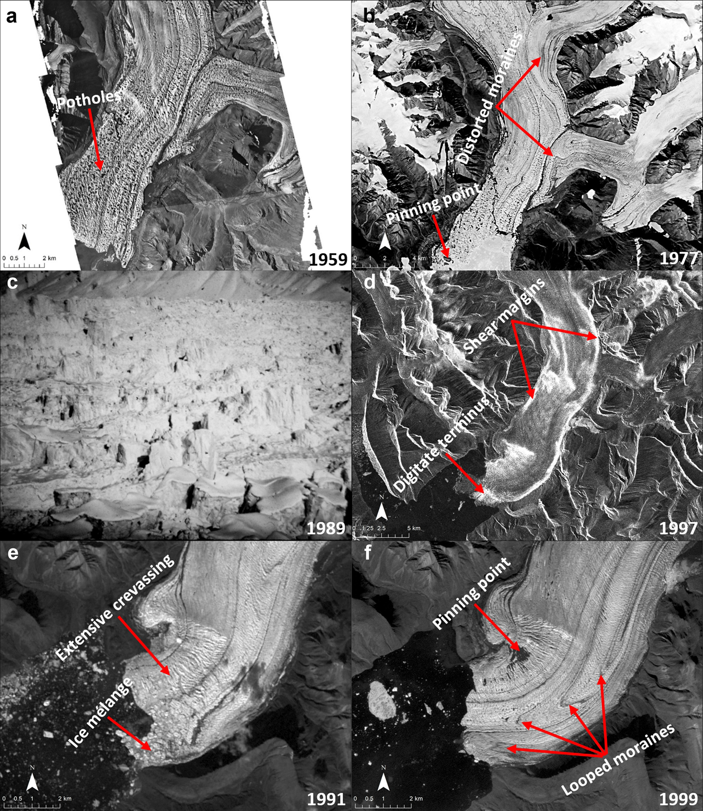
Fig. 3. Iceberg Glacier surface features indicative of surging. (a) Clearly visible extensive potholing on the glacier surface during quiescence. (b) 13 July 1977 KH-9 image showing distorted medial moraines at the junction between the two lower tributaries and the trunk and a pinning point in front of the terminus. (c) Low-altitude oblique aerial photograph taken in 1989 near the terminus showing that the glacier had a highly broken up surface (personal communication from M. Ecclestone, 2021). (d) Shear margins and splaying of the terminus onto the sea ice forming a digitate terminus, which can be observed from an 8 April 1997 ERS-1 SAR scene. (e) Landsat 5 image 9 August 1991 displaying extensive crevassing near the terminus and ice mélange at the ice front. (f) Medial moraines from the tributaries of Iceberg Glacier that were displaced far downstream by fast moving ice, creating looped moraines (25 July 1999, Landsat 7). The same pinning point as in (b) is also visible.
Conversely, the glacier had a heavily crevassed surface (Fig. 3e), large looped moraines (Fig. 3f) and clearly visible shear margins from SAR scenes in the 1990s (Fig. 3d). Moreover, a photograph taken during a flight from Expedition Fiord in 1989 (Fig. 3c) shows that Iceberg Glacier had a highly broken up surface (personal communication from M. Ecclestone, 2021), indicating that the glacier was flowing at a very rapid rate and that it had started surging before 1989. Sea ice and iceberg mélange was present at the glacier front in August–September 1980 and throughout 1981. This could be indicative of increased ice velocities and calving rates at the terminus of Iceberg Glacier in the early 1980s.
Meanwhile, the surge termination was inferred from optical and SAR imagery to have occurred in the early 2000s on account of the terminus retreat that started after 1997, and the progressive decrease in the extent of crevassing and shear margins. Ice surface velocities can help to further constrain the timing of surge initiation and termination, which are examined in the following section.
4.2 Velocity patterns
The surface velocities of Iceberg Glacier varied significantly throughout the study period as the glacier underwent a surge cycle. Here we describe broad trends in velocity without uncertainties, although our uncertainties range from <10 m a−1 for the most recent satellite observations to ~40 m a−1 for older datasets (Table 2). The mean centreline velocity of the trunk of Iceberg Glacier from 1972 to 1980 derived from Landsat 1–3 imagery was ~89 m a−1. Velocities reached >100 m a−1 from 14 to 23 km up-glacier from the 1997 terminus position, which roughly equates to the area between the junctions of the two lowermost tributaries with the trunk. Conversely, velocities near the terminus were typically below 50 m a−1, but appear to have generally increased throughout the 1970s, reaching values of >100 m a−1 in 1979–80. Although coverage of single image-pair velocities are often fairly poor, velocities downstream of 26 km from the 1997 terminus seem to have increased throughout this period (Fig. 4). Iceberg Glacier flowed at a median rate of 27 m a−1 (SD of 30 m a−1) over the entire trunk width downstream of 26 km, with a maximum velocity of 134 m a−1 in 1972–74 (Fig. 4). Over 1979–80, a median velocity of 95 m a−1 (SD of 41 m a−1) and a maximum velocity of 264 m a−1 was observed (Fig. 4), with the majority of the acceleration occurring within the terminus region.

Fig. 4. Evolution of the median and maximum surface velocities of Iceberg Glacier below 26 km from the 1997 terminus for 1972–80. Velocities were derived from feature-tracking on Landsat 1–3 imagery.
The flow rate within the terminus region of Iceberg Glacier underwent a drastic increase in summer 1981, with velocities reaching up to roughly 1500 m a−1 (Fig. 5). This represents a more than 50-fold increase in ice surface velocities in parts of the terminus region compared to the 1972–80 average. The velocities derived for 19 July 1981 to 30 August 1981 have large uncertainties, but manual tracking of features between these images reveals velocities at the terminus region reaching >1700 m a−1. This acceleration was accompanied by a ~100–400 m advance of the easternmost ~1.5 km of the terminus, where velocities attained >1000 m a−1. The marked increase in surface velocities observed in summer 1981, along with the appearance of ice mélange in front of the terminus in 1980, suggests that a surge likely started in the early 1980s.
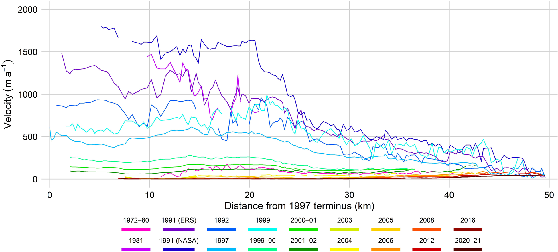
Fig. 5. Iceberg Glacier centreline (Fig. 1) surface velocities from 1972 to 2021, based on distance from the maximum terminus extent in 1997. Velocities for the period 1972–1980 represent the mean of several annually separated velocity scenes derived from feature-tracking. The velocity profiles prior to 1999 were extracted from Landsat 1–3, ERS-1/2 and NASA ITS_LIVE scene pairs, while all profiles since 1999 were derived from NASA ITS_LIVE (Gardner and others, Reference Gardner, Fahnestock and Scambos2019) scene pairs or annual mosaics.
Although velocities are unknown from 1982 to 1990 due to a lack of available imagery, results show particularly high velocities in 1991, indicating that Iceberg Glacier was certainly still surging at that time. The average centreline ice flow derived from June–July 1991 NASA ITS_LIVE image-pair velocities was 910 m a−1, with a maximum centreline value of approximately 1800 m a−1 (Fig. 5). Velocities of >2000 m a−1 were recorded over the northern half of the terminus with a highest value of 2320 m a−1. Ice flow along the centreline in summer 1991 remained above 1000 m a−1 within 24 km from the 1997 terminus position, constituting the year with the highest velocities on record. Meanwhile, average centreline velocities during fall 1991 quantified from a pair of ERS-1 scenes dropped to 690.3 m a−1, peaking at >1500 m a−1 at the terminus (Fig. 5). In the subsequent year, centreline velocities remained below 1000 m a−1 with a mean of 490.2 m a−1, which then further decreased to a mean velocity of 348.4 m a−1 in 1997 when 75% of the velocity profile remained below 500 m a−1 (Fig. 5).
The 1999 velocities were about 57% higher than in 1997, with a mean centreline velocity of 546.2 m a−1 and ice flow consistently greater than 500 m a−1 up to 26 km from the 1997 terminus position (Fig. 5). It is unclear whether this constitutes an actual speedup or whether the differences in velocities could be explained by the large median uncertainties of 89 m a−1 for 1991 and/or by the fact that velocities in 1997 were derived from spring (April–May) scenes, while the 1999 velocities were extracted from summer (July) images. During the surge, the distorted medial moraines found at the junction between the two lowermost tributaries and the trunk (Fig. 3b) were pushed toward the glacier margin by up to 1 km due the main trunk's rapid flow. Some medial moraines from these two tributaries were also displaced by the fast moving ice and brought several kilometres downstream to form looped moraines that are visible in optical imagery from the 1990s and early 2000s (Fig. 3f).
Thereafter, velocities showed a steady decrease from the beginning of the 21st century until present. The most drastic deceleration occurred between 1999 and 2000, when velocities dropped by a factor of three to an average of 189.5 m a−1 across the centreline (Fig. 5). This slowdown is in accordance with results extracted from RADARSAT-1 speckle tracking by Short and Gray (Reference Short and Gray2005), which showed that the flow rate of Iceberg Glacier had decreased to 75–130 m a−1 by fall 2000. The majority of the remaining slowdown during the transition to the quiescent phase occurred between 2000 and 2003. Centreline velocities dropped to an average of 132.9 m a−1 in 2000–01, followed by another drop to 94 m a−1 in 2001–02, and finally to 17 m a−1 in 2003 at a distance of approximately 7.5–15 km from the 1997 terminus (Fig. 6). By 2004, the average summer velocity was 39.1 m a−1 across the centreline while the terminus region was entirely stagnant (Fig. 6). This is also consistent with findings by Short and Gray (Reference Short and Gray2005), which show that the ice flowed at a rate of <25 m a−1 in midwinter 2004. This suggests that surge termination likely occurred in 2003.

Fig. 6. Iceberg Glacier centreline (Fig. 1) surface velocities from 2003 to 2021 showing the start of the quiescent phase of the surge cycle. All velocity profiles come from the NASA ITS_LIVE dataset. Distance from the terminus is based on the maximum terminus extent in 1997. Note difference in velocity scale from Fig. 5.
Contrary to the velocity profiles during the active phase of the surge where velocities were highest in the lower half of Iceberg Glacier and started decreasing upstream of ~20–25 km from its maximum surge terminus position (Fig. 5), velocities in the post-surge quiescent period were highest above 30 km from the terminus (Fig. 6). By 2009, velocities remained below 25 m a−1 across the entire glacier trunk, confirming the findings of Van Wychen and others (Reference Van Wychen2016, Reference Van Wychen2021) that the entire trunk had become essentially stagnant by ~ 2010. Velocities continued to decrease to values of <10 m a−1 over most of the glacier trunk within the last decade, and ice motion has been <50 m a−1 along the entire velocity profile since 2016 (Fig. 6). Since the end of the surge in 2003, the average centreline velocities of Iceberg Glacier have decreased from 39.1 m a−1 in 2004 to 11.5 m a−1 in 2020–21 (Fig. 6).
4.3 Elevation changes
While large changes in terminus position and variations in glacier velocities are evident manifestations of surging behaviour, patterns in ice surface elevation changes can indicate dynamic instabilities and are critical for glacier mass balance estimates. From 27 July 1959 to 13 July 1977, Iceberg Glacier experienced thickening over most of the main trunk and its upper tributary, while parts of the other tributaries and the trunks' lowermost 3–4 km thinned. Thickening was especially pronounced in the upper region of the trunk, with typical values ranging from approximately 4–6 ± 1.3 m a−1 and peaking at >7 ± 1.3 m a−1 (Fig. 7a), indicating that parts of the upper region of the glacier gained more than 100 ± 24.1 m of ice. Thinning rates reached roughly −7 ± 1.3 m a−1 on the eastern side of the terminus, but mainly remained below −3 ± 1.3 m a−1 (Fig. 7a). Elevation changes computed over bedrock shows a west to east pattern of thickening/thinning, with high positive uncertainties more common in the western portion of the DEM and high negative uncertainties more common in the eastern half. This pattern is pronounced at high elevations, and could be due to distortions in the DEMs. Uncertainties computed over bedrock vary between approximately −80 m (−4.4 m a−1) and 200 m (11.1 m a−1).
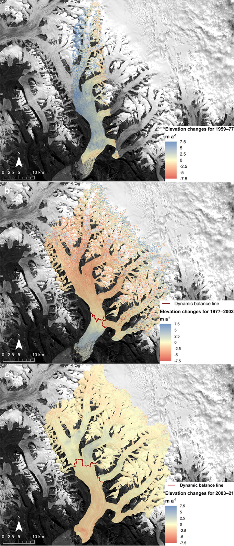
Fig. 7. Surface elevation change trends (m a−1) for Iceberg Glacier and its tributaries for the periods (a) 1959–77, (b) 1977–2003 and (c) 2003–21. Maps (a) and (c) represent elevation changes when the glacier was quiescent, while (b) roughly coincides with the timing of the active phase of the surge. The dynamic balance line is shown as a red line in (b) and (c). Base image: Landsat 8 composite image.
During the active phase, opposite elevation change trends were observed, with differencing of the 13 July 1977 KH-9 DEM and 26 May 2003 ASTER DEM showing ice thickness gains in the lower part of the glacier and losses in the upper part (Figs 7b, 8). This period roughly coincides with the active phase of the surge that lasted from approximately 1981 to 2003. Below 16 km from the 1997 terminus position, the glacier thickened at an average rate of 1.7 ± 1 m a−1 across the 10 m elevation bands of the glacier and experienced the most pronounced thickening of >3 ± 1 m a−1 at 7–12 km from the 1997 terminus (Fig. 8), reaching >80 ± 16.8 m in elevation gains over the 26-year period. The highest single-cell value of approximately 7 ± 1 m a−1 was recorded on the western side of the ice front (Fig. 8). The remainder of the surface of the main trunk and upper tributary at approximately 16–60 km from the 1997 terminus position lost, on average, 2 ± 1 m a−1 of ice across the 10 m hypsometric bands (Fig. 8).

Fig. 8. Mean glacier surface elevation change trends (m a−1) for Iceberg Glacier in each 10 m elevation band for the periods 1977–2003 (active phase; blue) and 2003–21 (quiescent phase; red). The distance from the terminus is based on the maximum terminus extent in 1997. The black solid vertical line indicates the location of the 1977–2003 dynamic balance line and the black dashed vertical line shows the location of the 2003–21 dynamic balance line.
After 2003, the elevation change patterns reversed once again, reflecting the accumulation of mass at high elevations. The gains in surface elevation occurred between approximately 32 and 49 km from the 1997 terminus position at a mean rate of 0.6 ± 0.4 m a−1 along the 10 m hypsometric bands (Fig. 8), and at a maximum single-cell rate of about 3 ± 0.4 m a−1 at ~42.5 km (Fig. 7c). Meanwhile, the elevation bands downstream of ~32 km from the 1997 terminus position lost mass at an average rate of 1.1 ± 0.4 m a−1 (Fig. 8), and the terminus region encountered the most substantial thinning, reaching mean single-cell rates over the entire 2003–21 period as high as nearly −5 ± 0.4 m a−1 (Fig. 7c) at ~8 km from the 1997 terminus. These patterns persisted throughout the current quiescent period, although the magnitude of the elevation changes appears to have decreased since 2003, and the patterns were less apparent in 2015–21 in comparison to the previous twelve years.
The dynamic balance line (DBL) represents the location separating the reservoir zone from the receiving zone and encounters no net change in surface elevation (Dolgoushin and Osipova, Reference Dolgoushin and Osipova1975; Kochtitzky and others, Reference Kochtitzky2019). The DBL is inferred to be at ~15.5–20 km from the 1997 terminus position (~200 m a.s.l.) during the surge (Figs 7b, 8), and between approximately 30 and 33 km from the 1997 terminus position across the main trunk (~400 m a.s.l.) during the current quiescent phase (Figs 7c, 8).
5. Discussion
An abrupt terminus advance, an increase in surface velocities, formation of new crevasses and/or surface elevation changes are all indicators of a possible surge initiation (Meier and Post, Reference Meier and Post1969; Raymond, Reference Raymond1987; Sund and others, Reference Sund, Eiken, Hagen and Kääb2009; Kochtitzky and others, Reference Kochtitzky2019). Therefore, the marked increase in ice flow in 1981, the >7 km terminus advance that occurred between 1981 and 1997, as well as the crevasses, shear margins and looped moraines visible on the glacier in the 1990s strongly suggests that a surge occurred with a likely initiation in the early 1980s. Surge termination occurred in 2003 when the average surface velocity over the lowermost ~7.5 km of the glacier dropped to below 20 m a−1 (Fig. 5).
5.1 Mass redistribution
Iceberg Glacier exhibited a surface evolution marked by a net movement of mass down-glacier during the active phase of the surge with high velocities, followed by an accumulation of mass over the upper part of the glacier during quiescence and a period of low velocities. To assess the relative importance of glacier dynamics vs surface mass balance (SMB) in accounting for the surface elevation changes observed over the glacier, SMB data from Noël and others (Reference Noël2018) were used for the periods 1958–95 and 1996–2015, derived with the regional climate model RACMO2.3 (https://doi.pangaea.de/10.1594/PANGAEA.881315). SMB is defined as the difference between the processes adding mass to a glacier surface (e.g., precipitation, drifting snow) and those removing mass (e.g., melt, runoff, sublimation), and in this study were determined for every 50 m elevation band across the trunk of Iceberg Glacier and upper tributary (Fig. 2d). The geodetic mass balance data extracted from the 1977 KH-9 and 2003–21 ASTER DEMs were downsampled to 1 km to match the resolution of the SMB data, and the dynamic mass balance was computed by subtracting the SMB from the geodetic mass balance. Therefore, the dynamic mass balance represents the total elevation change resulting from the vertical movement of ice and variations in glacier dynamics, and does not take into account elevation change due to changes in surface mass. Volume changes per 50 m elevation band were then calculated by multiplying the median elevation change (i.e., geodetic mass balance) of each band by the band's area. The SMB data were converted from water equivalent to ice equivalent values using a density of 850 ± 60 kg m−3, following Huss (Reference Huss2013). The median SMB values over each elevation band from 1958 to 1995 were used for 1977–2003 (active phase), while the median 1996–2015 values over each elevation band were used for 2003–21 (quiescent phase).
The SMB data showed negative values up to elevations of 600–650 m a.s.l. (~43 km from the 1997 terminus) and an average ice loss of 1.0 ± 0.2 m a−1 across the entire glacier surface for 1958–95. SMB values from 0–400 m a.s.l. for that period averaged a negative mass balance of −2 ± 0.2 m a−1, which reduced the amplitude and upstream extent of positive geodetic mass balance changes during the surge; Iceberg Glacier thickened and gained mass geodetically up to an elevation of 150–250 m a.s.l. (<20 km from the 1997 terminus) compared to 350–400 m a.s.l. (>25 km from the 1997 terminus) dynamically (Fig. 9a). The rate of thickening over the 50–100 m a.s.l. elevation band peaked at values of 3.3 ± 1.0 m a−1 (5.1 ± 1.0 m a−1 dynamically), equivalent to a volume gain of 0.07 ± 0.001 km3 a−1 (Fig. 9a). Conversely, the glacier experienced the greatest rate of thinning by −5.2 ± 1.0 m a−1 at an elevation of 600–650 m a.s.l., but saw the greatest volume loss of −0.06 ± 0.001 km3 a−1 over the 350–400 m a.s.l. elevation band due to its largest area of 26.4 km2.
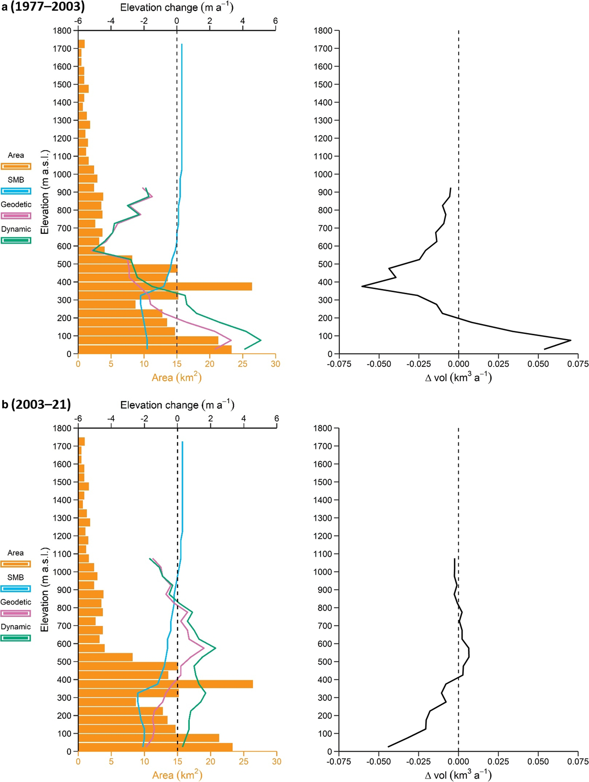
Fig. 9. Iceberg Glacier median ice surface elevation change (geodetic mass balance), surface mass balance (SMB) and dynamic balance for each elevation band (left), and the median ice volume loss per elevation band (right), during: (a) the active phase (1977–2003) and (b) the quiescent phase (2003–21). Glacier area in each 50 m elevation band (hypsometry) derived from 2001–21 mean.
The 1996–2015 SMB data reveal more negative mass balance conditions over Iceberg Glacier than in 1958–95, with an average value of −1.4 ± 0.2 m a−1 over the main trunk and the upper tributary (Fig. 2d), and an up-glacier extension of the SMB equilibrium line altitude from 600–650 m a.s.l. (~43 km from the 1997 terminus) in 1958–95 to 950–1000 m (~54 km from the 1997 terminus) in 1996–2015. As before, geodetic mass balance changes were generally more negative due to the inclusion of SMB, and the dynamic mass balance suggests that the glacier thickened at an average rate of 1.0 ± 0.4 m a−1 up to an elevation of 950–1000 m a.s.l. Fig. 9b).
Geodetic mass loss during quiescence does not necessarily reflect the climatic mass balance of surge-type glaciers because the ablation area can be dynamically refilled from an area above the reservoir zone immediately after a surge (Gardelle and others, Reference Gardelle, Berthier, Arnaud and Kääb2013; Kochtitzky and others, Reference Kochtitzky2019), leading to a positive dynamic mass balance in this region. In the case of Iceberg Glacier, mass being added to the trunk from the upper parts of tributaries, which have maintained a higher flow rate than the trunk during quiescence, could perhaps explain some of the observed dynamic thickening. Positive geodetic mass balance and volume changes for 2003–21 both peaked at an elevation of approximately 500–600 m a.s.l. at values of 1.6 ± 0.4 m a−1 and 0.007 ± 0.0004 km3 a−1, respectively (Fig. 9b). Higher elevations (>800 m a.s.l.) thinned, possibly due to a continuing drawdown of mass driven by the relatively high velocities that were sustained over the upper regions of the tributaries throughout the quiescent phase. In fact, the upper three tributaries of Iceberg Glacier appear to play a key role in refilling the reservoir zone during quiescence owing to their relatively high flow rates and, consequently, high rates of mass transfer.
Summing of the volume changes for all elevation bands for the 1977–2003 active phase indicates that a total geodetic mass gain of 4.3 ± 0.1 km3 of ice occurred over the lower 200 m elevation band of Iceberg Glacier, compared to a total mass loss of 8.0 ± 0.4 km3 over the rest of the surface, equivalent to a glacier-wide mean annual mass balance of −0.14 ± 0.02 km3 a−1. During the quiescent phase to date (2003–21), the glacier has gained a total of 0.5 ± 0.1 km3 of ice from 400–800 m a.s.l. and lost a total of 2.9 ± 0.1 km3 of ice in the receiving zone below 400 m a.s.l., equivalent to a mean volume loss across the main trunk and upper tributary of −0.15 ± 0.01 km3 a−1. For a surge-type glacier in a negative mass balance state, the change in glacier hypsometry characterised by the movement of large quantities of ice mass to lower, warmer elevations during a surge event can result in an overall more negative mass balance. The similarity in mean annual geodetic mass balance between the active and quiescent phases, however, suggests that changes in total mass of Iceberg Glacier are dominated by long-term negative surface mass balance conditions, irrespective of surge phase.
5.2 Length of the active phase and surge mechanisms
Surge initiation is inferred to have occurred in 1980 or 1981 based on the formation of ice mélange in front of the terminus, a marked increase in surface velocities in summer 1981, and the significant terminus advance that ensued. The surge likely terminated in 2003 as centreline velocities reached an average of 17 m a−1 over the lowermost 7.5 km of the glacier, although velocities continued to decrease over the entire glacier during the following >10 years (Fig 6). Consequently, it is likely that Iceberg Glacier surged for a total of ~22 years.
Previous studies on glaciers located in Svalbard and parts of Greenland have shown that surge initiation and termination can occur over several years (Mouginot and others, Reference Mouginot, Bjørk, Millan, Scheuchl and Rignot2018), but that surge initiation tends to happen much more rapidly than surge termination (Murray and others, Reference Murray, Strozzi, Luckman, Jiskoot and Christakos2003), which seems to be the case for Iceberg Glacier. However, Iceberg Glacier was flowing at a much faster rate in 1972–80 than during its current quiescent period, which raises the question of whether the glacier started accelerating prior to the 1970s. In fact, Iceberg Glacier was flowing at virtually the same average rate from 1972 to 1980 as during the end of the active phase in 2001–02, and following a similar pattern, with both years having average centreline velocities of ~90 m a−1 (Fig. 5). Additionally, our velocity results show a gradual increase in flow rates from 1972 to 1980 that, despite the poor spatial coverage of image-pair velocities derived from Landsat 1–3 images, appear to have resulted in more than a tripling of median velocities within 26 km from the 1997 terminus (Fig. 4), particularly within the terminus region. Nevertheless, the glacier did not appear have any surface features indicative of surging throughout the 1970s, such as new crevasses, suggesting that the glacier was likely not actively surging during that period. Instead, it seems that surface velocities on Iceberg Glacier had been gradually increasing since at least the early 1970s before the primary surge-triggering event that occurred in the early 1980s. The main tributaries of Iceberg Glacier, and particularly the lowermost two tributaries, were flowing at much higher rates in 1972–80 near their junction with the trunk than they presently are, with velocities reaching up to approximately 200 m a−1. It has been shown that ice motion generally increases downstream of the junction between a glacier tributary and trunk (e.g., Gudmundsson, Reference Gudmundsson1999), which seems to have occurred for the lower two tributaries of Iceberg Glacier for 1972–80, where average centreline velocities of >100 m a−1 were found between 14 and 23 km from the 1997 terminus. Therefore, the higher velocities during the 1970s in comparison to the current quiescent phase could be at least partly related to tributary dynamics.
The drivers of glacier surging have been generally separated into two categories based on basal processes, with surge initiation either prompted by a build-up of water pressure at the glacier bed due to the collapse of subglacial channels as ice overburden pressure increases during quiescence (Alaska-type surges; Kamb and others, Reference Kamb1985) or by a switch from cold to temperate basal conditions due to an increase in ice thickness during quiescence (Svalbard-type surges; Clarke, Reference Clarke1976; Murray and others, Reference Murray, Strozzi, Luckman, Jiskoot and Christakos2003). Hydrologically-regulated Alaska-type surges occur in regions with relatively temperate climates such as Alaska and Yukon, have shorter surge cycles and typically higher velocities than thermally-regulated Svalbard-type surges that are generally found in colder, drier climates, such as Svalbard and the Canadian Arctic (Murray and others, Reference Murray, Strozzi, Luckman, Jiskoot and Christakos2003). For example, surge-type glaciers in Svalbard experience surge cycles of 50–500 years and active phases of 3–15 years (Dowdeswell and others, Reference Dowdeswell, Hamilton and Hagen1991, Reference Dowdeswell, Hodgkins, Nuttall, Hagen and Hamilton1995), while a glacier in Alaska has been shown to have a surge recurrence interval of just 5 years (Nolan and others, Reference Nolan, Kochtitzky, Enderlin, McNabb and Kreutz2021). Alaska-type surges are also subject to a much shorter surge initiation and termination on the order of days to months (Kamb and others, Reference Kamb1985; Murray and others, Reference Murray, Strozzi, Luckman, Jiskoot and Christakos2003).
Iceberg Glacier, with its active phase of more than 20 years, seemingly long quiescent phase length, and slow surge termination, seem to best fit under the category of a thermally-regulated surge. Nevertheless, there is a wide range of observed surge behaviour that do not properly fit in one of the two proposed categories of surges, including combined thermo-hydrological triggers, making the distinction between the two suggested surge mechanisms unclear in certain instances (Dunse and others, Reference Dunse2015; Sevestre and others, Reference Sevestre2018; Benn and others, Reference Benn2019b; Haga and others, Reference Haga2020).
In an attempt to unify different surge mechanisms through a single framework, Benn and others (Reference Benn, Fowler, Hewitt and Sevestre2019a) proposed a general theory of surging that uses enthalpy as a universal unit through which ice flow instabilities can be studied. Enthalpy quantifies the internal energy of a glacier system that is primarily a function of ice temperature and water content (Aschwaden and others, Reference Aschwanden, Bueler, Khroulev and Blatter2012; Benn and others, Reference Benn, Fowler, Hewitt and Sevestre2019a). Enthalpy is gained at the glacier bed through geothermal heating, frictional heating and the supply of meltwater. Meanwhile, enthalpy losses occur through heat conduction from the bed to the glacier surface and drainage of meltwater (Benn and others, Reference Benn, Fowler, Hewitt and Sevestre2019a). When balances in both enthalpy and mass flux are not met, this prevents the glacier from remaining in a stable steady state by periodically increasing mass flux to evacuate the buildup of excess enthalpy at the glacier bed (Sevestre and Benn, Reference Sevestre and Benn2015; Benn and others, Reference Benn, Fowler, Hewitt and Sevestre2019a).
In the CAA, low basal enthalpy production and efficient conductive heat losses from cold atmospheric temperatures typically does not favour surging (Sevestre and Benn, Reference Sevestre and Benn2015). However, glaciers that are long, branchy, and cover large areas are less likely to find a balance between enthalpy production and enthalpy losses than small, simple glaciers because they tend to have higher balance velocities and, as a result, higher basal enthalpy production at the bed (Sevestre and Benn, Reference Sevestre and Benn2015). In addition, larger glaciers tend to be thicker, which reduces the capability of the glacier to evacuate enthalpy by conductive heat losses to the atmosphere (Sevestre and Benn, Reference Sevestre and Benn2015). Unlike some smaller glaciers, larger glaciers may also be unable to evacuate cumulative water discharge via inefficient, distributed subglacial drainage systems, leading to increased basal water storage and velocity-strain heating feedbacks (Sevestre and Benn, Reference Sevestre and Benn2015). The large total basin size of Iceberg Glacier (~1000 km2), low surface slope, high length and large altitude range fit the geometric profile of surge-type glaciers in the CAA (Sevestre and Benn, Reference Sevestre and Benn2015). Testing whether the observed sequence of events of surge-type glaciers in this region match predictions made by the enthalpy balance model could be achieved by quantifying key elements of the enthalpy budget at different stages of the surge (Benn and others, Reference Benn2019b), providing a compelling avenue for future work. The following sub-section will examine potential mechanisms that could have triggered the surge.
5.3 Location of surge initiation
The presence of ice mélange at the glacier front in 1980–81, the high (>1000 m a−1) velocities recorded over the terminus region in 1981, and the ~100–400 m advance of the easternmost ~1.5 km of the terminus between 1980 and 1981, strongly suggests that the surge of Iceberg Glacier initiated at the terminus. Up-glacier surge propagation from the terminus accompanied by extensional crevassing has been reported several times for tidewater surge-type glaciers in Svalbard (e.g., Rolstad and others, Reference Rolstad, Amlien, Hagen and Lundén1997; Luckman and others, Reference Luckman, Murray and Strozzi2002; Dowdeswell and Benham, Reference Dowdeswell and Benham2003; Murray and others, Reference Murray, Strozzi, Luckman, Jiskoot and Christakos2003; Flink and others, Reference Flink2015; Sevestre and others, Reference Sevestre2018). Sevestre and others (Reference Sevestre2018) suggest that during the late quiescent phase, internal thermodynamic processes resulting from the gradual steepening of the glacier surface, such as a velocity-strain heating feedback and/or retreat from a pinning point, leads to the acceleration of the glacier front and the development of terminal crevasse fields. Crevasses then channel meltwater and rainwater to the glacier bed, resulting in flow acceleration and an upward migration of the crevasse field, which coincides with surge propagation (Sevestre and others, Reference Sevestre2018).
The westernmost ~2 km of the terminus of Iceberg Glacier was located on a bedrock pinning point in 1981, which is visible as a rock ridge in front of the terminus (Fig. 3b), while the rest of the terminus had retreated by more than 2 km from that bedrock perturbation. The centre part of the bedrock ridge is also clearly visible in 2014 radio-echo sounding data, at ~7 km up-glacier from the 1997 terminus (Fig. 10). The retreat of a marine-terminating glacier from a pinning point into deeper water has been shown to increase thinning and retreat rates, while increasing ice velocities (O'Neel and others, Reference O'Neel, Pfeffer, Krimmel and Meier2005; Sevestre and others, Reference Sevestre2018), as part of what has been termed the tidewater glacier cycle (Meier and Post, Reference Meier and Post1987). In this cycle, grounded tidewater glaciers may undergo long periods of very slow advance, followed by shorter periods of rapid disintegration and retreat accompanied by high ice velocities. While this process could have driven the large retreat of the eastern part of the terminus from 1959 to 1981, it cannot explain the rapid terminus advance during its high flow event from 1981 to 2003, followed by stagnation.
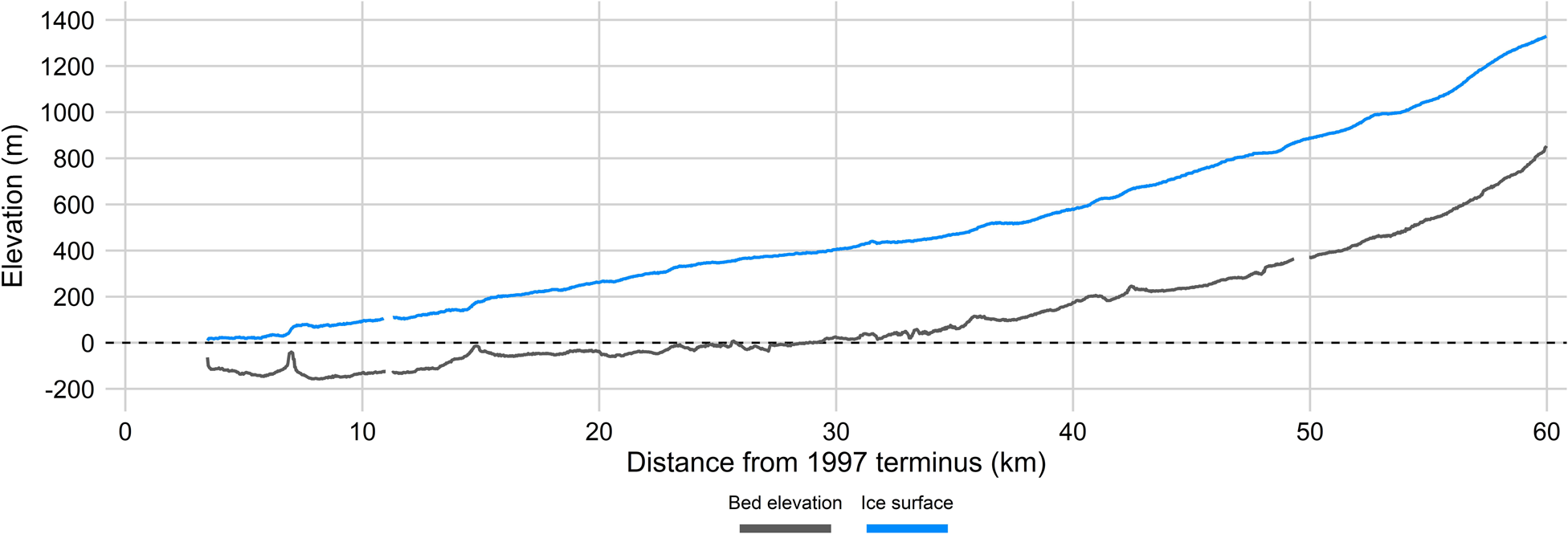
Fig. 10. Ice surface (blue) and bed elevation (dark grey) profiles extracted along the centreline from 3D tomography radio-echo sounding data (https://data.cresis.ku.edu/) collected by NASA Operation IceBridge on 25 March 2014.
Substantial thinning of the terminus region results in an increase in buoyancy until the terminus reaches flotation, which is, in turn, followed by an acceleration of ice flow (O'Neel and others, Reference O'Neel, Pfeffer, Krimmel and Meier2005). To determine whether Iceberg Glacier was close to flotation near the start of its surge, we used the following equation presented in Cuffey and Paterson (Reference Cuffey and Paterson2010) to quantify the thickness in excess of flotation by comparing the ratio of ice thickness to water depth:

where H M is total ice thickness, ρ w is the density of water, ρ i is the density of ice, and H w is water depth. H M was computed by subtracting the absolute bed elevation from the surface elevation of the glacier, while the absolute bed elevation was used to determine H w. NASA Operation IceBridge 3D tomography radio-echo sounding data (https://data.cresis.ku.edu/) from 2014 was used for the bed elevation, while the 1977 KH-9 DEM and a 2016 ArcticDEM tile were used for the surface elevation. Flotation is likely to occur in areas where H b approaches 0 or is negative.
The data from Iceberg Glacier shows that the majority of the ice front in 1977 had H b values below 0, and reaching as low as approximately −30 m (Fig. 11a). While the KH-9 DEM has relatively high vertical uncertainties, and negative elevation values over parts of the terminus are possibly due to the presence of deep potholes, these results suggest that a large part of the terminus had reached flotation by 1977. The westernmost portion of the terminus remained far from flotation (up to ~25 m from flotation; Fig. 11a) due to the presence of the bedrock perturbation, which reaches elevations of up to ~100 m above sea level and stabilised that part of the terminus during the quiescent phase. That portion of the terminus also saw a much less pronounced acceleration in 1981 than the eastern portion, overall lower velocities during the active phase due to the compressional flow, increased driving stress resulting from the higher surface slope due to the bedrock perturbation and significantly less thinning than the eastern side of the terminus from 1959 to 1977 (Fig. 7a). Considering the west to east pattern in elevation change values over bedrock described in section 4.3, which is albeit less prominent near the terminus than at higher elevations, part of this spatial change in thinning rates at the terminus could be the result of uncertainties. Downstream from the bedrock pinning point, the glacier switched to extensional flow during the surge, leading to extensive transverse crevassing (Fig. 3e).
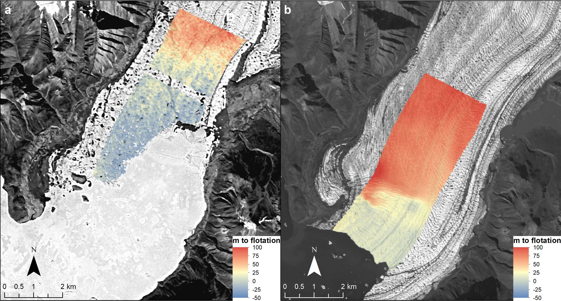
Fig. 11. Thickness in excess of flotation for the terminus region of Iceberg Glacier in: (a) 1977 and (b) 2016 quantified by comparing the ratio of ice thickness to water depth (Eqn 3). Ice thickness and water depth was derived from 3D tomography radio-echo sounding data (https://data.cresis.ku.edu/) collected by NASA Operation IceBridge on 25 March 2014 along with an (a) KH-9 DEM and (b) ArcticDEM tile. Base images: (a) KH-9, 13 July 1977 and (b) Landsat 8, 29 July 2016.
In comparison, the terminus of Iceberg Glacier was significantly less likely to float in 2016, with typical values of >10 m of thickness in excess of flotation (Fig. 11b). Fundamentally, the lower ice thickness and deeper fiord waters over which the eastern half of the terminus was located in 1977 would have increased its buoyancy. Ice mélange developed between 6 July 1980 and 30 August 1980 as sea ice appears to have thinned and retreated from part of the glacier front during that period, which would have caused a reduction in buttressing at the terminus and could account for some of the coincident increase in ice movement and calving (Pimentel and others, Reference Pimentel2017). Sea ice did not fully retreat from the glacier front in 1980, but in 1981 sea ice fully disappeared from Iceberg Bay between 19 July and 30 August, during which time the terminus region underwent a dramatic acceleration.
However, hydrologic forcing has been shown to play a more important role than frontal buttressing by sea ice or ice mélange in the intra-annual dynamics of Belcher Glacier, on Devon Island (Pimentel and others, Reference Pimentel2017). The modelled mass balance of White Glacier (~35 km east of Iceberg Glacier) for 1981 is slightly negative (Thomson and others, Reference Thomson, Zemp, Copland, Cogley and Ecclestone2017), and in 1981 the northern CAA had the highest annual mean temperature anomaly since at least 1958 of ~1.25°C with respect to the 1958–95 period (Noël and others, Reference Noël2018). It is likely that these relatively high temperatures would have resulted in an increased availability of meltwater within the glacier system during the summer months, some of which would have been routed to the glacier bed through crevasses. This, in turn, has been shown to increase the area of the glacier bed that is subject to cryo-hydraulic warming from the refreezing of surface water and basal hydraulic lubrication, resulting in a hydro-thermodynamic feedback (Dunse and others, Reference Dunse2015). Ultimately, positive air temperatures coupled with significant surface to bed drainage routed via crevasses can result in rapid acceleration and contribute to surge initiation as evidenced by some tidewater terminating glaciers in Svalbard (e.g., Dunse and others, Reference Dunse2015; Sevestre and others, Reference Sevestre2018; Benn and others, Reference Benn2019b).
When the sequence of observed changes at Iceberg Glacier are put together, a likely sequence for the surge initiation is as follows: (1) more than half of the terminus of Iceberg Glacier had retreated from a bedrock pinning point by 1966 and more than two thirds by 1981, which enhanced further retreat and increased extension, resulting in higher thinning rates and velocities; (2) gradual steepening of the glacier surface throughout the quiescent period likely caused an increase in internal and basal temperatures within the reservoir zone as well as an increase in driving stress; (3) probable flotation of a large portion of the eastern terminus of Iceberg Glacier occurred in the 1970s; (4) the complete retreat of sea ice from the ice front in summer 1981 for the first time since September 1978 removed a buttressing force at the terminus, which could have contributed to the surge initiation of Iceberg Glacier; and (5) the relatively warm air temperatures of 1981 (Noël and others, Reference Noël2018) likely increased water availability at the glacier bed through routing of meltwater via crevasses, which could have been another important mechanism in the rapid acceleration of the terminus measured during that year. Further channelling of meltwater to the glacier bed as more crevasses developed following surge initiation probably played a role in the up-glacier propagation of the surge from the terminus as described by Sevestre and others (Reference Sevestre2018), although we lack sufficiently high spatial and temporal resolution data to confirm this.
5.4 Comparison to other surge-type glaciers in the CAA
Besides Iceberg Glacier, the two other largest outlet glaciers on western Axel Heiberg Island, Airdrop Glacier (~600 km2; land-terminating) and Good Friday Glacier (~800 km2; marine-terminating), have also been previously classified as surge-type (Müller, Reference Müller1969; Copland and others, Reference Copland, Sharp and Dowdeswell2003). These glaciers were deemed to be subject to surging behaviour based on the presence of surface features diagnostic of surging activity, such as large looped moraines, heavy crevassing, significant terminus advance over the period 1959–99 and high ice surface velocities (Copland and others, Reference Copland, Sharp and Dowdeswell2003). However, neither Good Friday Glacier nor Airdrop Glacier have shown any cyclic variations in their dynamics characteristic of surge-type glaciers since observations began in the 1950s. Instead, both glaciers appear to have continuously advanced over the last seven decades and have maintained relatively high velocities during that period (Medrzycka and others, Reference Medrzycka, Copland, Van Wychen and Burgess2019; Lauzon and others, Reference Lauzon, Copland, Van Wychen, Kochtitzky and McNabbin review). Yet, the highest measured velocity of ~2300 m a−1 at the terminus of Iceberg Glacier in summer 1991 is more than an order of magnitude higher than the highest flow rate on record for Airdrop Glacier (Lauzon and others, Reference Lauzon, Copland, Van Wychen, Kochtitzky and McNabbin review). Nevertheless, both Good Friday Glacier and Airdrop Glacier have started slowing down nearly synchronously since the mid-2000s. Good Friday Glacier decelerated by ~50–100 m a−1 over that period (Medrzycka and others, Reference Medrzycka, Copland, Van Wychen and Burgess2019), while Airdrop Glacier slowed down by a factor of ~2.3 between 2006 and 2020–21 within 7 km from its 2018 terminus position (Lauzon and others, Reference Lauzon, Copland, Van Wychen, Kochtitzky and McNabbin review). This deceleration has been interpreted as a possible slow transition to the quiescent phase of the surge cycle that spans more than a decade (Medrzycka and others, Reference Medrzycka, Copland, Van Wychen and Burgess2019; Van Wychen and others, Reference Van Wychen2021; Lauzon and others, Reference Lauzon, Copland, Van Wychen, Kochtitzky and McNabbin review), although alternate explanations for both glaciers' behaviour have been proposed, including a delayed response to positive mass balance conditions of the Little Ice Age and an unstable advance related to perturbations in the bedrock topography of Good Friday Glacier (Medrzycka and others, Reference Medrzycka, Copland, Van Wychen and Burgess2019; Lauzon and others, Reference Lauzon, Copland, Van Wychen, Kochtitzky and McNabbin review).
If Good Friday Glacier and Airdrop Glacier are indeed surging, their several-decade-long active phase would likely fall under the category of a slow surge (Jiskoot, Reference Jiskoot, Singh, Singh and Haritashya2011; Lauzon and others, Reference Lauzon, Copland, Van Wychen, Kochtitzky and McNabbin review). Slow surges typically last longer than an ordinary surge with an active phase of >20 years, are subject to lower flow speeds and sometimes result in no change in terminus position (Jiskoot, Reference Jiskoot, Singh, Singh and Haritashya2011). Split Lake Glacier, a land-terminating glacier located on SE Ellesmere Island that has been actively surging for 50+ years and flowing at a velocity reaching >600 m a−1, is the first to have been classified as a slowly surging glacier in the Canadian Arctic (Van Wychen and others, Reference Van Wychen, Hallé, Copland and Gray2022). Considering the active phase length of ~22 years, its significant terminus advance of ~7 km and sudden acceleration to velocities of >1500 m a−1, Iceberg Glacier appears to best fit under the category of a classical (i.e., ‘normal’) surge rather than a slow surge.
Other glaciers in the CAA have been shown to experience classical surges, which is best exemplified by the dynamics of Otto Glacier and Mittie Glacier on Ellesmere Island. Otto Glacier was reported by Hattersley-Smith (Reference Hattersley-Smith1964, Reference Hattersley-Smith1969) to be undergoing a surge in 1963–64 that began between 1950 and 1959 and reached a maximum measured velocity of 7.7 m d−1 (equivalent to 2800 m a−1) in July–August 1959. The glacier was experiencing surge-like velocities of >800 m a−1 again in 1991, which dropped to <50 m a−1 in 2013–15. This suggests an active phase length of at least 22 years (Millan and others, Reference Millan, Mouginot and Rignot2017; Van Wychen and others, Reference Van Wychen2021). Assuming that the surge event observed between 1950 and 1964 is not the same as the one observed between 1991 and 2013, these observations suggest a surge recurrence interval of <30 years.
Mittie Glacier, located on SE Ellesmere Island, was actively surging in 1999, with surface velocities of 1000 m a−1 over its entire 25 km length (Copland and others, Reference Copland, Sharp and Dowdeswell2003) and continued high velocities of up to ~1000 m a−1 at the terminus in 2003 and ~700 m a−1 in 2004 (Short and Gray, Reference Short and Gray2005). The glacier had reached stagnation by 2012, suggesting an active phase length of at least 5 years (Van Wychen and others, Reference Van Wychen2014). Ultimately, CAA glaciers appear to experience long surges when compared to the active phase length of 3–10 years for surge-type glaciers in Svalbard (Dowdeswell and others, Reference Dowdeswell, Hamilton and Hagen1991) and a generally slow transition from the active phase to the quiescent phase of the surge cycle. The length of the active phase for surge-type glaciers in the Canadian Arctic appears to vary between anywhere from >5 years to possibly >70 years, indicating that there exists a wide range of complex surge behaviour and dynamics within this region.
6. Conclusions
By combining remotely sensed data from a variety of sources from 1950 to 2021, our results support previous observations that suggested cyclic variations in the dynamics of Iceberg Glacier (Copland and others, Reference Copland, Sharp and Dowdeswell2003; Short and Gray, Reference Short and Gray2005; Van Wychen and others, Reference Van Wychen2016), thus confirming its surge-type classification. Iceberg Glacier experienced a prolonged period of terminus retreat from 1950 to 1980, during which time the glacier was in the quiescent phase and ice velocities remained relatively low. However, median velocities appear to have gradually increased from 1972 to 1980, most notably over the eastern portion of the terminus between 1979 and 1980, while the westernmost ~2 km remained grounded on a bedrock pinning point. Ice mélange appeared at the glacier front in summer 1980 and was accompanied by an acceleration in ice movement within the terminus region of Iceberg Glacier, which reached up to ~1500 m a−1 when the active phase of the surge began in August 1981. We hypothesise that retreat of the terminus from a bedrock pinning point, internal thermodynamic processes, terminus flotation, the removal of the buttressing force exerted by sea ice, and an increase in subglacial meltwater from high air temperatures, all likely played a role in surge initiation at the terminus of Iceberg Glacier.
The 1981–2003 surge resulted in a total terminus advance of >7 km in 1997 compared to pre-surge extent in 1980, a peak velocity of ~2300 m a−1 in summer 1991, and a large drawdown of mass from regions up-glacier of the DBL causing pronounced thickening at the terminus. During the current quiescent phase, a high rate of terminus retreat has been accompanied by a long-term decrease in surface velocities to an average centreline value of 11.5 m a−1 in 2020–21. Surface elevation trends show mass accumulation over the upper reservoir zone of the glacier and mass loss over the lower receiving zone.
This study provides the first detailed reconstruction of an entire surge for a glacier in the Canadian Arctic and reveals insights into the mechanisms that drive surging in this region. We conclude that the surge of Iceberg Glacier most closely resembles a thermally-triggered Svalbard-type surge, although hydrological changes at the glacier bed through channelling of meltwater via crevasses could also play an important role in regulating surging (e.g., Dunse and others, Reference Dunse2015; Sevestre and others, Reference Sevestre2018; Benn and others, Reference Benn2019b; Haga and others, Reference Haga2020). If Airdrop Glacier and Good Friday Glacier are indeed surge-type, it would be puzzling as to why two nearby surge-type glaciers would behave this differently from Iceberg Glacier, with an active phase length of possibly more than 3 times that of Iceberg Glacier. Additional research is needed to understand the precise mechanisms causing certain glaciers to undergo long-term advances and/or slow surges, while other glaciers of similar geometries and subject to similar environmental conditions undergo shorter, more intense surges.
Acknowledgements
This work was supported by funding from the Natural Sciences and Engineering and Research Council (NSERC) of Canada, ArcticNet Network of Centres of Excellence Canada, University of Manitoba and University of Ottawa. We thank the National Air Photo library for their help with acquiring some of the historical aerial photographs for Iceberg Glacier. We are grateful to the Canadian Space Agency (CSA) and NASA for obtaining the MCoRDS ice penetrating radar data over the glacier. The tomography radar data products were generated by CReSIS (Center for Remote Sensing of Ice Sheets) with support from the University of Kansas, NASA Operation IceBridge grant NNX16AH54G and NSF grant ACI-1443054. We would also like to thank GAMMA Remote Sensing for their help with the processing of ERS data.


 Open access