SRRF: A Beginners Guide

Introduction

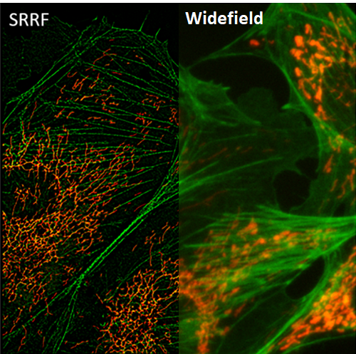
Super-resolution radial fluctuations (SRRF) is a super-resolution algorithm that analyzes radial and temporal fluorescence intensity fluctuations in an image sequence to generate a super‑resolution image. Broadly speaking, SRRF works because we know that noise is uncorrelated in time whereas fluorophores are. By combining spatial and temporal information from multiple images, SRRF can produce images with resolution approaching ~60 nm. For details on how SRRF works, please refer to our full application note.

The SRRF algorithm, developed by Henriques and colleagues (2016), is a freely available ImageJ plugin that allows anyone to use the technique on any camera. The ImageJ-based GPU-enabled post-processing SRRF algorithm is named NanoJ-SRRF.

**Figure 1:** Comparison of widefield and SRRF image on BPAE cells with stained mitochondria (red) and actin (green)

Installing NanoJ-SRRF

NanoJ-SRRF can be downloaded and installed from the latest version of ImageJ or Fiji and can be found here.

Open ImageJ
Go to Help, then Update. This opens the ImageJ Updater
Select ‘Manage Update Sites’ to open a list of sites that host ImageJ plugins
As seen in Fig. 2, pick NanoJ-SRRF from the list. You can also access other plugins from the NanoJ set, including NanoJ-Core and NanoJ-SQUIRREL. Select the desired plugins and then Close the window.
The ImageJ Updater will show the plugins to install, select Apply Changes, and then restart ImageJ. NanoJ-SRRF is now installed as an ImageJ plugin.

**Figure 2:** Available sites that host ImageJ plugins, navigate to N and find the NanoJ collection.

Starting NanoJ-SRRF

Once installed, NanoJ-SRRF can be used to analyze any preexisting image in a format that can be opened in ImageJ.

NanoJ-SRRF can be accessed from the Plugins menu within ImageJ (Fig. 3).

In this menu, you can access the SRRF algorithm to analyze images with the ‘SRRF Analysis’ option, as well as access Advanced Settings (which can also be accessed from SRRF Analysis menu), and the ability to check the NanoJ-SRRF version, updates and website.

To perform analysis, select ‘SRRF Analysis’. This will open options for SRRF analysis, as seen in Fig. 4.

**Figure 3:** Once installed, NanoJ-SRRF can be accessed from the Plugins menu. Select ‘SRRF Analysis’ or ‘Configure Advanced Settings’ to begin analysis.

**Figure 4:** *Left* Analysis options and *Right* Advanced settings for SRRF analysis. Default settings are currently selected on both.

The windows shown in Fig.4 show the options for SRRF analysis and the ability to access the advanced settings. These settings can be optimized depending on the application and the nature of the image. A full explanation of these settings can be found in the manual but some of the more important ones will be discussed here.

To start running SRRF on a dataset, select SRRF Analysis. You will then be prompted to load an image stack to analyze. A good SRRF image will need a stack of ~100 images to produce one SRRF image, but generally the more frames of data the better the final image.

SRRF Analysis

It is important to first realize how SRRF works to understand how changing the analysis parameters will affect the image.

The first thing that needs to be understood is that SRRF works by breaking down each pixel in every frame of the image stack into ‘subpixels’ (Fig. 5).

Each subpixel is then assigned a value related to the probability that it contains a fluorophore. This is done by measuring local radial symmetries in the image (the ‘radiality’).

The radiality is a measurement of intensity gradient convergence: For every subpixel, intensity gradient vectors are measured for a ring of nearby surrounding subpixels. The degree of convergence of these vectors at the original central subpixel is then calculated. For a subpixel located close to the true center of an individual fluorescent molecule, there will be a high degree of convergence and hence a high radiality value. In this way, radiality infers the molecule position. This radiality measurement is performed on every image in the stack to generate a radiality stack (Culley et al. 2018).

**Figure 5:** Subpixels created from image pixels.
Adapted from Culley *et al.* 2018

The radiality transform gives the spatial information. The temporal information is then needed to generate the final SRRF image which is why it’s important to have a lot of frames of data.

When plotting the radiality value over time, the temporal fluctuation shows whether the subpixel is centered on a fluorophore or not. The degree of temporal correlation tells us with greater precision where the fluorophore is more likely to be in the image.

SRRF Analysis Parameters

Once the image stack is loaded in, the SRRF Analysis dialog box will populate with the default settings. It may be worth running the algorithm on default settings first to see the impact on the image before adjusting the parameters.

Some of the key parameters and what they do are outlined below.

Ring Radius

Ring radius sets the radius of the ring used to calculate the intensity gradient vectors of nearby surrounding subpixels. It follows that the highest resolution will be obtained with the smallest ring, however, in busy or noisy data a small ring will reduce precision and may introduce patterning. Generally, the lower the density of the data, the smaller the ring radius can be but high-density data may need a larger ring radius for best results. In SRRF the default value is a ring radius of 0.5, the impact of changing the ring radius can be seen in Fig.6.

Radiality Magnification

The radiality magnification sets how may subpixels the original image pixels should be split into. To use 5×5 subpixels like in Fig.4, the radiality magnification should be set to 5. Generally, the more subpixels there are the better the resolution will be. However, the more subpixels there are, the greater the computational time needed to run the algorithm. A value of 5 is recommended to start, the impact of changing the radiality magnificiation can be seen in Fig.7.

Axes In Ring

The radiality is calculated in a ring around a subpixel, the radius of which is determined by the ring radius. The axes in ring determine the number of points around the circumference of this ring that are used in the calculation. The higher the value, the greater the fidelity of the data but at the cost of increased computational time. It’s not recommended to reduce this value below the default, which is 6. The impact of changing the axes can be seen in Fig.7.

Advanced Settings

The advanced settings dialog box gives more control over the temporal analysis side of the algorithm, the calculation of the radiality transform and weighting.

Temporal Radiality Maximum (TRM) displays the final image as a maximum intensity projection (good for low-density images).

Temporal Radiality Average (TRA) displays the final image as an average intensity projection (good starting point for all analysis).

Temporal Radiality Pairwise Product Mean (TRPPM) displays the final image as the raw second moment of the radiality over the time series (similar to TRA with additional noise suppression)

Temporal Radiality Auto-Correlations (TRAC) performs auto-correlation analysis similar to that used in the SOFI (good for high-density images)

The remaining advanced settings are all optimizations for different types of images being used which might benefit from certain adjustments.

Summary

SRRF is an extremely useful super-resolution algorithm, and making use of it is easier than ever thanks to NanoJ-SRRF and the ability to use SRRF for images taken with back-illuminated sCMOS cameras.

References

Culley, S., Toshevaab, K. L., Pereira, P. M. & Henriques, R. (2018) Universal live-cell super-resolution microscopy. The International Journal of Biochemistry & Cell Biology. Volume 101, Pages 74-79. https://doi.org/10.1016/j.biocel.2018.05.014

Gustafsson N., Culley S., Ashdown G., Owen D.M., Pereira P.M., Henriques R. (2016) Fast live-cell conventional fluorophore nanoscopy with ImageJ through super-resolution radial fluctuations, Nature Communications, 7, 12471, DOI: 10.1038/ncomms12471