Differentialgleichungen
Differentialgleichungen
Differentialgleichungen

You also want an ePaper? Increase the reach of your titles
YUMPU automatically turns print PDFs into web optimized ePapers that Google loves.
<strong>Differentialgleichungen</strong><br />
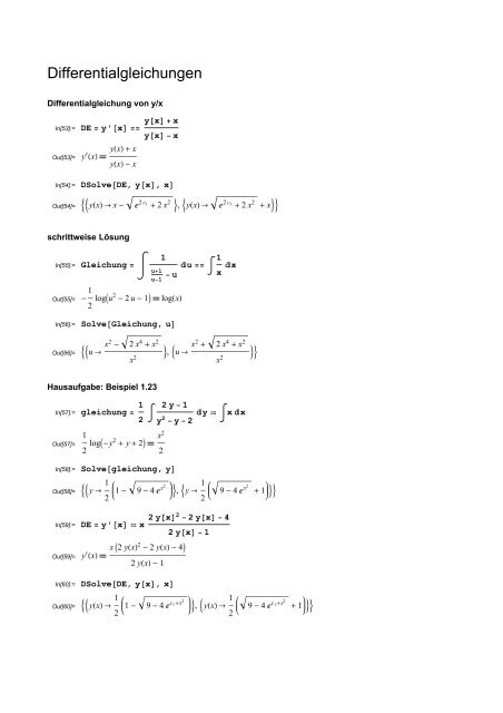
Differentialgleichung von y/x<br />
In[53]:= DE = y'@xD ==<br />
Out[53]= y £ yHxL + x<br />
HxL <br />
yHxL - x<br />
y@xD + x<br />
y@xD − x<br />
In[54]:= DSolve@DE, y@xD, xD<br />
Out[54]= ::yHxL Ø x - ‰ 2 c 1 + 2 x 2 >, :yHxL Ø ‰ 2 c 1 + 2 x 2 + x>><br />
schrittweise Lösung<br />
In[55]:= Gleichung = ·<br />
1<br />
u+1<br />
− u<br />
u−1<br />
Out[55]= - 1<br />
2 logIu2 - 2 u - 1M logHxL<br />
In[56]:= Solve@Gleichung, uD<br />
Out[56]= ::u Ø x2 - 2 x 4 + x 2<br />
x 2<br />
Hausaufgabe: Beispiel 1.23<br />
u == ‡<br />
1<br />
x x<br />
>, :u Ø x2 + 2 x 4 + x 2<br />
In[57]:= gleichung = 1<br />
2 ‡<br />
2y− 1<br />
y2 − y − 2 y ‡ x x<br />
Out[57]=<br />
1<br />
2 logI-y2 + y + 2M x2<br />
In[58]:= Solve@gleichung, yD<br />
Out[58]= ::y Ø 1<br />
2<br />
2<br />
1 - 9 - 4 ‰x2<br />
>, :y Ø 1<br />
2<br />
In[59]:= DE = y'@xD x 2y@xD2− 2y@xD− 4<br />
2y@xD− 1<br />
Out[59]= y £ HxL x I2 yHxL2 - 2 yHxL - 4M<br />
2 yHxL - 1<br />
In[60]:= DSolve@DE, y@xD, xD<br />
Out[60]= ::yHxL Ø 1<br />
2 1 - 9 - 4 ‰c1+x2 x 2<br />
9 - 4 ‰ x2<br />
>, :yHxL Ø 1<br />
2<br />
>><br />
+ 1 >><br />
9 - 4 ‰ c1+x2 + 1 >>
2 MatheIII03-.nb<br />
In[61]:= DSolveB:y'@xD x 2y@xD2− 2y@xD− 4<br />
,y@x0D y0>, y@xD, xF<br />
2y@xD− 1<br />
Solve::ifun :<br />
Inverse functions are being used by Solve, so some solutions may not be found;<br />
use Reduce for complete solution information. à<br />
Solve::ifun :<br />
Inverse functions are being used by Solve, so some solutions may not be found;<br />
use Reduce for complete solution information. à<br />
Out[61]= ::yHxL Ø 1<br />
2 1 - 9 - I-4y02 + 4y0+ 8M ‰ x2-x02 >, :yHxL Ø 1<br />
2<br />
In[62]:= DSolveB:y'@xD x 2y@xD2− 2y@xD− 4<br />
,y@0D 3>, y@xD, xF<br />
2y@xD− 1<br />
9 - I-4y0 2 + 4y0+ 8M ‰ x2 -x0 2<br />
Solve::ifun :<br />
Inverse functions are being used by Solve, so some solutions may not be found;<br />
use Reduce for complete solution information. à<br />
Solve::ifun :<br />
Inverse functions are being used by Solve, so some solutions may not be found;<br />
use Reduce for complete solution information. à<br />
DSolve::bvnul : For some branches of the general solution,<br />
the given boundary conditions lead to an empty solution. à<br />
Solve::ifun :<br />
Inverse functions are being used by Solve, so some solutions may not be found;<br />
use Reduce for complete solution information. à<br />
General::stop :<br />
Further output of Solve::ifun will be suppressed during this calculation. à<br />
Out[62]= ::yHxL Ø 1<br />
2<br />
16 ‰ x2<br />
+ 9 + 1 >><br />
In[63]:= DirectionField@DE_, y_@x_D, 8x_, a_, b_
MatheIII03-.nb 3<br />
In[64]:= plot1 = DirectionField@DE, y@xD, 8x, −2, 2
4 MatheIII03-.nb<br />
Out[65]=<br />
General::stop :<br />
Further output of Solve::ifun will be suppressed during this calculation. à<br />
DSolve::bvnul : For some branches of the general solution,<br />
the given boundary conditions lead to an empty solution. à<br />
DSolve::bvnul : For some branches of the general solution,<br />
the given boundary conditions lead to an empty solution. à<br />
DSolve::bvnul : For some branches of the general solution,<br />
the given boundary conditions lead to an empty solution. à<br />
General::stop :<br />
Further output of DSolve::bvnul will be suppressed during this calculation. à<br />
Part::partw : Part 1 of 8< does not exist. à<br />
ReplaceAll::reps :<br />
88
MatheIII03-.nb 5<br />
In[66]:= Show@plot1, plot2, PlotRange → 80, 5
6 MatheIII03-.nb<br />
In[69]:= FullForm@%D<br />
Out[69]//FullForm=<br />
List@List@Rule@y@xD, Plus@-1, Times@-2, ProductLog@Times@Rational@-1, 2D,<br />
Power@Power@E, Plus@-1, Times@-1, xD, Times@-1, C@1DDDD, Rational@1, 2DDDDDDDD,<br />
List@Rule@y@xD, Plus@-1, Times@-2, ProductLog@Times@Rational@1, 2D,<br />
Power@Power@E, Plus@-1, Times@-1, xD, Times@-1, C@1DDDD, Rational@1, 2DDDDDDDDD<br />
In[70]:= ? ProductLog<br />
ProductLog@zD gives the principal solution for w in z we w .<br />
ProductLog@k, zD gives the k th solution. à<br />
Zum Schluss noch ein Beispiel, bei welchem Mathematica fälschlicherweise keine korrekte<br />
Fallunterscheidung vornimmt.<br />
In[71]:= DE = y'@xD x 1 + y@xD<br />
Out[71]= y £ HxL x yHxL + 1<br />
In[72]:= DSolve@DE, y@xD, xD<br />
Out[72]= ::yHxL Ø 1<br />
16 I4 c1 x 2 2 4<br />
+ 4 c1 + x - 16M>>
MatheIII03-.nb 7<br />
In[73]:= plot1 = DirectionField@DE, y@xD, 8x, −5, 5
8 MatheIII03-.nb<br />
In[75]:= Show@plot1, plot2, PlotRange → 8−1, 5><br />
1
MatheIII03-.nb 9<br />
à Beispiel 1.12<br />
In[78]:= DSolve@y'@xD Sin@xD y@xD, y@xD, xD<br />
Out[78]= 99yHxL Ø c1 ‰ -cosHxL ==<br />
In[79]:= DSolve@8y'@xD Sin@xD y@xD, y@0D 1
10 MatheIII03-.nb<br />
Diese einfache Differentialgleichung für K[x] können wir aber durch Integration lösen und wir<br />
erhalten<br />
In[100]:= spezielleLösung = y@xD → KExpB‡ −a@xD xF ∗ ‡ b@xD ExpB‡ a@xD xF xO<br />
Out[100]= yHxL ؉ -Ÿ aHxL „x ‡ bHxL ‰ Ÿ aHxL „x „ x<br />
Test:<br />
In[101]:= test = DE ê. 8spezielleLösung, D@spezielleLösung, xD<<br />
Out[101]= True<br />
DSolve kann dies auch alleine, liefert aber wieder eine kompliziert aussehende Lösung.<br />
In[102]:= DSolve@DE, y@xD, xD<br />
Out[102]= ::yHxL ؉ Ÿ x x<br />
-aHK@1DL „K@1D<br />
1<br />
‡1 bHK@2DL ‰ -Ÿ<br />
K@2D<br />
-aHK@1DL „K@1D<br />
1<br />
„ K@2D + c1 ‰ Ÿ x<br />
-aHK@1DL „K@1D>><br />
1<br />
Beispiel 1.16<br />
In[103]:= DE = y'@xD y@xD + x<br />
Out[103]= y £ HxL yHxL + x
MatheIII03-.nb 11<br />
In[104]:= plot1 = DirectionField@DE, y@x D, 8x, −5, 5
12 MatheIII03-.nb<br />
In[106]:= plot2 = PlotB<br />
Out[106]=<br />
Evaluate@Table@y@xD ê. DSolve@8DE, y@0D k
MatheIII03-.nb 13<br />
In[107]:= Show@plot1, plot2, PlotRange → 8−5, 5< D<br />
Out[107]=<br />
4<br />
2<br />
0<br />
-2<br />
-4<br />
nach unserer Formel:<br />
In[108]:= a =−1; b = x;<br />
-4 -2 0 2 4<br />
Allgemeine Lösung der homogenen Differentialgleichung:<br />
In[109]:= hom = y1 → K ∗Ÿ−a x<br />
Out[109]= y1 Ø K ‰ x<br />
Variation der Konstanten:<br />
In[110]:= ‡ b Ÿ a x x<br />
Out[110]= ‰ -x H-x - 1L<br />
Spezielle Lösung der inhomogenen Differentialgleichung:<br />
In[111]:= var = y2 → Ÿ −a x ∗ ‡ b Ÿ a x x<br />
Out[111]= y2 Ø-x - 1<br />
Allgemeine Lösung der inhomogenen Differentialgleichung:
14 MatheIII03-.nb<br />
In[112]:= lösung = y → y1 + y2 ê. 8hom, var<<br />
Out[112]= y Ø K ‰ x - x - 1<br />
Wir lösen das Anfangswertproblem mit y(x0)=y0:<br />
In[113]:= Solve@Hlösung@@2DD ê. 8x → x0